Frugal machine learning for minimal hardware
Published on Aug 16, 2024 by Impaktor.
She’s a totally logical computer, a thing, that’s not a woman.
Star Trek TOS S1E7 - “What little girls are made of” (1966)
Note: These are my notes to myself on the general theme on how to reduce computational requirements for LLM/ML models.
Table of Contents
- 1. Introduction
- 2. Quantization - reduce precision
- 3. Pruning - reduce nodes
- 4. Knowledge distillation (model distillation)
- 5. Engineering / hardware integration
- 6. Appendix
1. Introduction
There are many frameworks (lama.cpp, ollama, vLLM, TGI, RayLLM) for serving a pre-trained language model locally. The training cost has already been paid. However, the training cost - although large - is a one time expense, and given time, it will be eclipsed by inference cost, which is carried by the end user.
Herein, I aim to explore the different strategies for reducing the hardware requirements (RAM, CPU, GPU) for running machine learning inference, on CPU (or GPU), (possibly explained assuming non-technical background).
It is assumed the reader is familiar with basics of neural networks, e.g. understands there’s a matrix with weights that are determined through the training procedure.
2. Quantization - reduce precision
There are currently many popular qunatized models available on Huggingface,
mainly by TheBloke (recommend Q5_K_M models, where K_M is usually
slightly better than K_S)
2.1. Numbers represented as bits
Consider an integer, e.g. 0, 1, 2, or 3. It is internally represented by a
set number of bits in the computer. With two bits, we can represent the
unsigned (positive) integers 0,1,2,3 (00, 01, 10, 11). Given one
more bit that determines if the integer is positive or negative, we can now
represent signed integers.
For a full precision floating point number, like float32 (4 bytes), we
partition the 32 bits into three parts:
- sign
- with
0corresponds to positive and1to negative number. - exponent
- a number of bits (e.g. 8) are reserved for representing the exponent
- mantissa
- the remaining of the bits (e.g. 23) are used for the significand, meaning representing the significant digits. The precision of the number depends on the number of bits used to represent it.
See this for in depth explanation, and huggingface blogpost on quantization on ML.
Thus we can represent numbers like (using base 10):
- \(61000 \rightarrow 1 \times 6.1 \times 10^{4}\)
- \(-0.0061 \rightarrow -1 \times 6.1 \times 10^{-3}\).
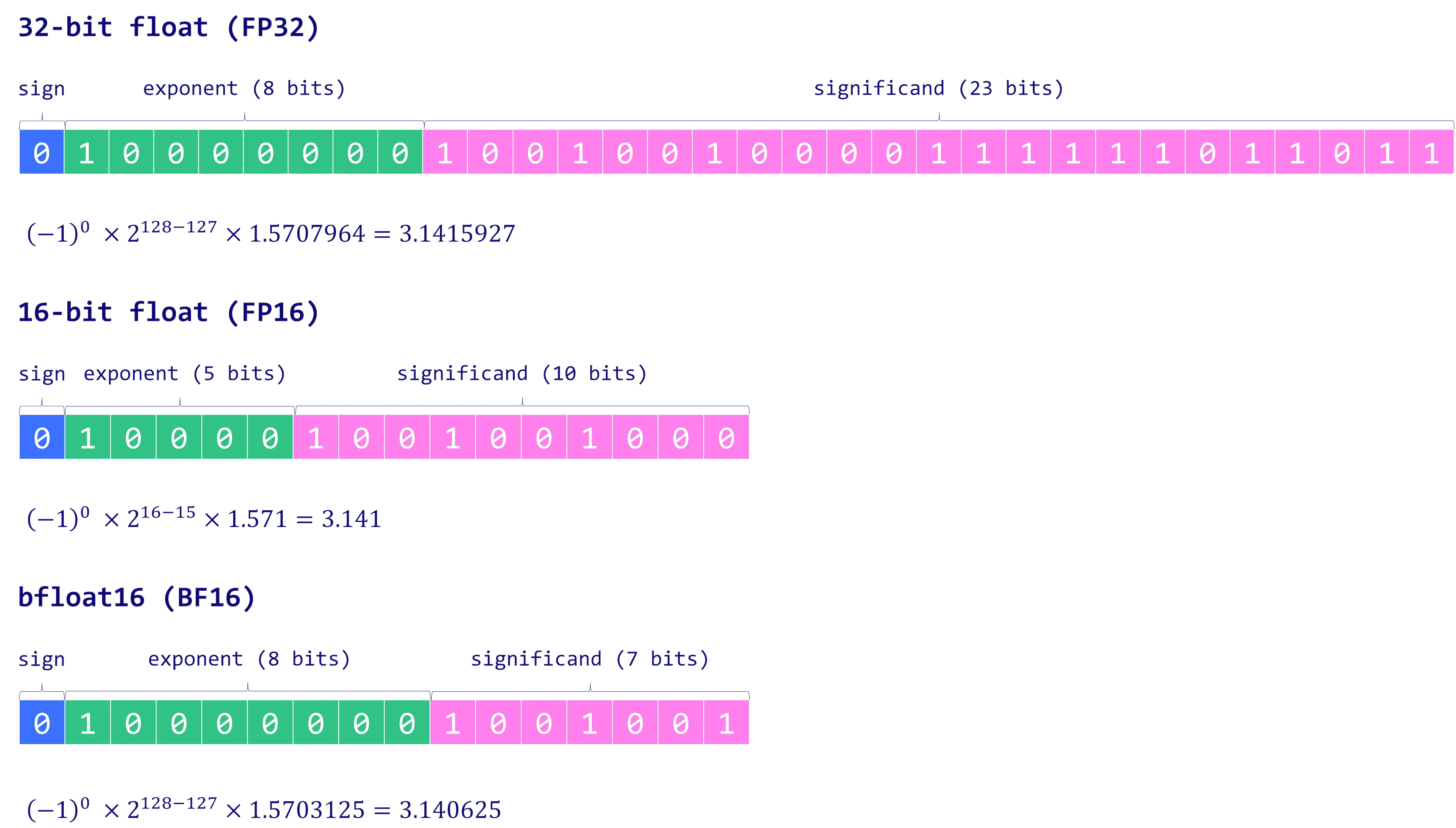
Figure 1: BF16 has greater range, but lower precision that FP16 [src].
2.2. Same number with fewer bits
A model like LLaMA2 has 7 billion parameters, thus with 32 bit float, it takes \(\frac{7 \times 10^9 \times 32 }{ 8 \times 10^9}=28\) GB of disk space. If we would express each parameter using fewer bits, it would save resources.
Rather than allocating 64 bits (float64) or 32 bits (float32) full
precision for each element in the weight matrix, we can map them to fewer,
like float16 (half precision) or int8, with no significant loss of
precision.
Note: speed gain e.g. from float32 to int8 depends on GPU. For some
there might be no difference, though typically one should aim to get 4 X
gain. Ideally, this is combined with a reduced precision execution engine.
2.3. Quantization algorithms:
There are several ways to map the higher numbers to lower quantization. At the most fundamental level, there are two base cases:
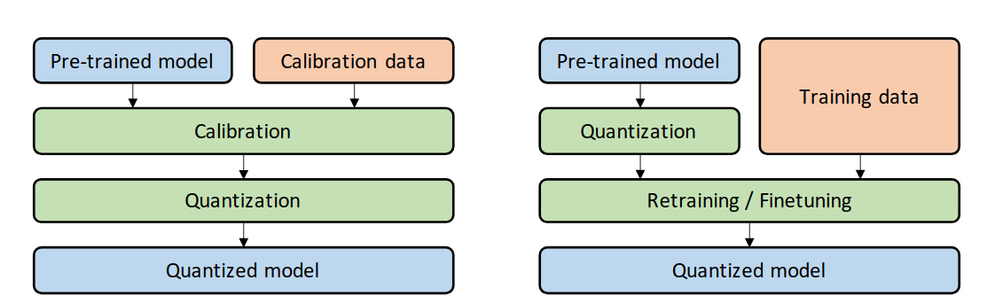
Figure 2: PTQ (left) and QAT (right). [src]
- PTQ
- Post-Training Quantization, where the weights are already trained, and then cast to lower bit representation.
- QAT
- Quantization-Aware Training, where quantization is done pre-training, or during fine-tuning, resulting in less performance loss, at the cost of computation. This can be done by inserting quantization & de-quantization between each layer, thus the cost function adapts to it, e.g. by selecting a minima that is broader / less sensitive to the exact value of the weights.
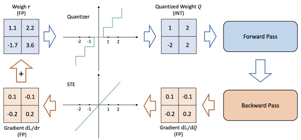
Figure 3: Quantization-Aware Training procedure. [src]
2.3.1. Absmax quantization
Map original number to range [-127, 127] (for int8). Maps \(0
\rightarrow 0\).
- scale factor is: \(\frac{127}{\max(|X|)}\)
- quantify: \(X_q = \text{scale} \times X\)
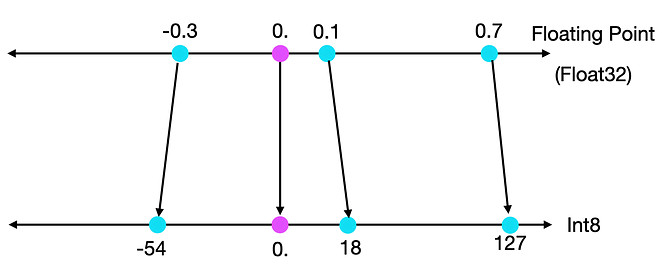
Figure 4: Absmax mapping [src]
2.3.2. Zeropoint quantization
Allow for asymmetric input distribution, by scaling it to the total range of the min & max values of the distribution. This makes use of the full range of available bits, from -128 to +126.
- scale factor is: \(s = \frac{255}{\max(X) - \min(X)}\)
- zeropoint is: \(z = -\text{round}(s \times \min({X})) - 128\)
- quantify: \(X_q = \text{round}(s \times X + z)\)
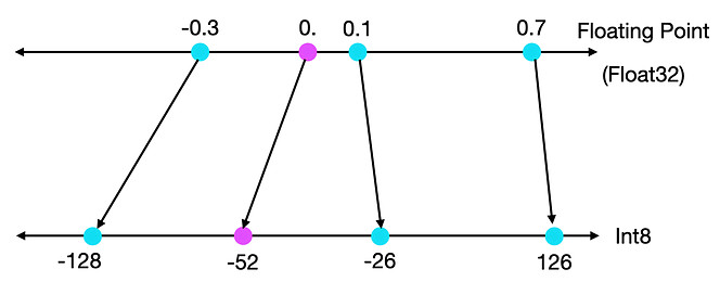
Figure 5: Zeropoint mapping [src]
2.4. Quantize weights vs activation?
Which to quantize?
2.4.1. Weight quantization
Only quantize storage, not computation
- Store weights as
int8, de-quantize tofloat32when running - Storage space gain, no speed gain (still
float32for computation)
2.4.2. Activation quantization:
Everything in quantized space.
- Convert all input and outputs to
int8, and also do computation inint8 - Faster (on most hardware)
- Since input is unknown during quantization, need calibration of scale
factor for each layer, or we will get clipping (values outside
int8range) in the hidden layers.
2.5. Extreme quantization
If we can reduce a float32 or even a float64 model to int8 model with
maintained precision, then the obvious question is:
- How much further can we quantize a floating precision model?
We glean possible answer:
- The paper BitNet: Scaling 1-bit Transformers for Large Language Models
(arXiv), they train a model (from scratch) to one bit weights
({
-1,1}), significantly reducing memory and energy consumption, while maintaining a performance comparable to its floating precision counterpart. The paper The Era of 1-bit LLMs: All Large Language Models are in 1.58 Bits (arXiv) explores using a ternary bit ({
-1,0,1}) weights by adding in the0(i.e.log(3)/log(2)bits). They write:[It] retains the benefits of the original 1-bit BitNet, including its new computation paradigm, which requires almost no multiplication operations for matrix multiplication and can be highly optimized. Additionally, it has the same energy consumption as the original 1-bit BitNet and is much more efficient in terms of memory consumption, throughput and latency compared to FP16 LLM baselines.
There are pre-trained models on HuggingFace Llama 1 bit and 2 bit models
2.6. Quantizing speed
Different quantization strategies vary greatly in speed and hardware requirements, some taking many hours, others only minutes, depending on if we need to re-train the model or if we can simply operate on the weights. In general, weight quantization comes in two flavors:
- Data-free calibration
- (e.g. bitsandbytes), using only the weights, and
- Calibration-based
- (e.g. GPTQ, AWQ), relying on external dataset (risk of introducing bias, and are computationally heavy). AWQ is the latest, and assumes not all weights are of equal importance, to gain inference speed up
Large models like Mixtral-8x7B perform well under 2-bit quantization. However, smaller models like Llama-2-7B do not respond as well to the same treatment, and quantizing down to single bit significantly reduces performance further.
Some quantization methods take hours (depending on zero-shot or one-shot), where e.g. Half-Quadratic Quantization (HQQ), (github) can quantize an LLM in minutes, while BitNet trains the full network from scratch. Furthermore, reducing the Llama-2-7B to 2 bit using HHQ+, yields a model that can outperform the full precision model(!) e.g. on GSM8K (8.5K high quality linguistically diverse grade school math word problems).
Authors behind HQQ+ note:
On one hand, training smaller models from scratch offers the advantage of reduced computational requirements and faster training times. Models such as Qwen1.5 have shown promising results and can be attractive options for certain applications. However, our findings indicate that heavily quantizing larger models using techniques like HQQ+ can yield superior performance while still maintaining a relatively small memory footprint.
2.7. Outliers
Most of the weights of each layer are distributed around the mean. However,
when we use a quantization algorithm like absmax in the presence of
outliers, they will compress the range for most weights such that most are
put in the same bin (of the 8 bins, assuming int8 quantization), such that we
can no longer distinguish them.
The outlier problem tends to grow for larger models with more parameters that are to fit into same number of bins. The result is the quantized weights for both outliers and non-outliers will have large error.
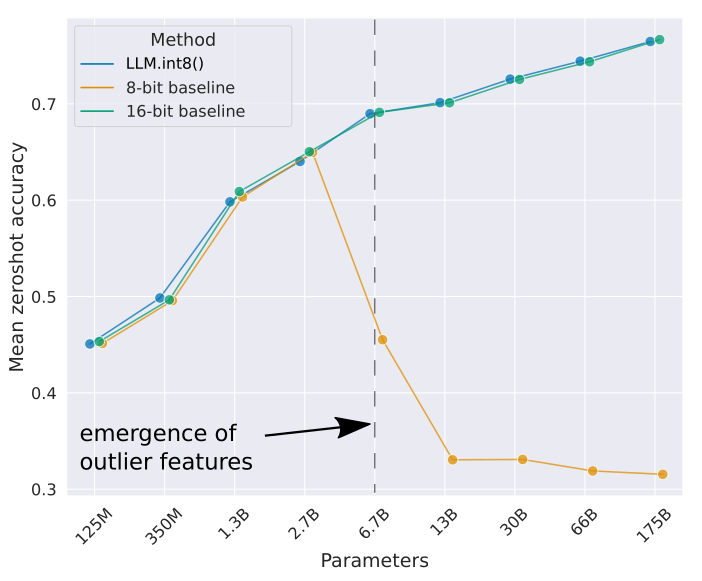
Figure 6: LLM.int8(): Fixed bins can’t store all values as number of parameters increases
This is alleviated by treating outliers separately as float16, as
demonstrated in the paper LLM.int8(): 8-bit Matrix Multiplication for
Transformers at Scale (arXiv):
- Given a threshold, extract outliers from input matrices
- Multiply non-outliers using
int8vector-wize quantization - Dequantize
int8tofloat16and add to outlier matrix.
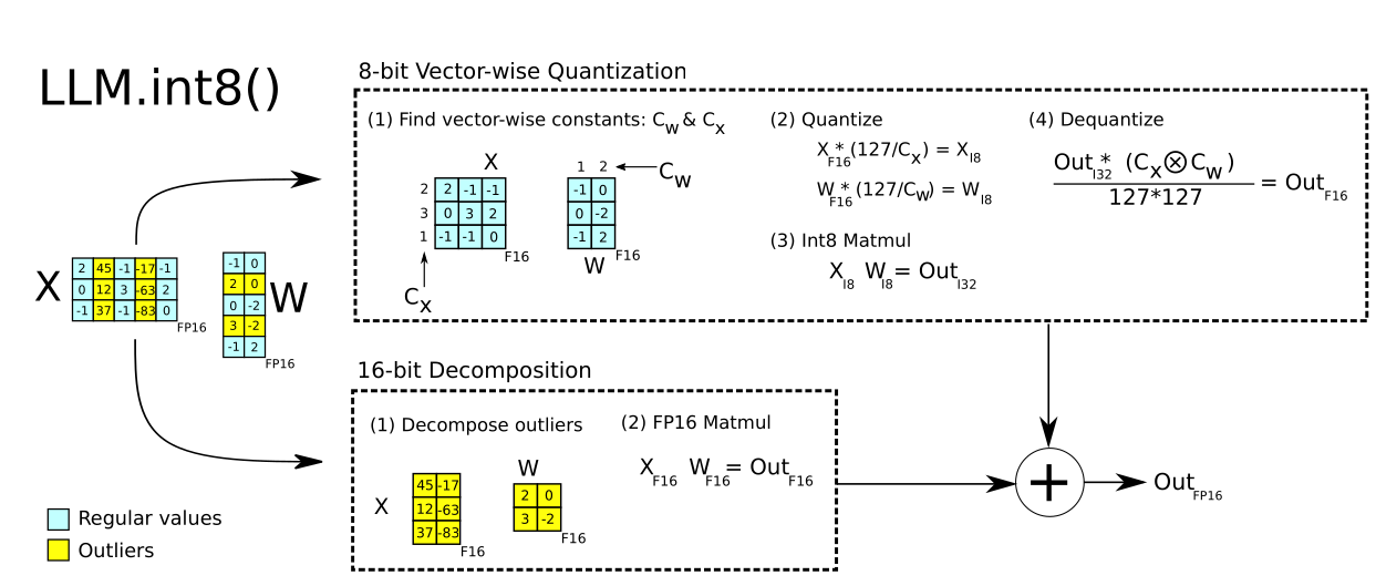
Figure 7: LLM.int8(): int8 in combination with float16 for outliers (yellow)
2.8. TODO Layer-by-layer quantization aware distillation
ZeroQuant: Efficient and Affordable Post-Training Quantization for Large-Scale Transformers, (arXiv) 2022
- Initialize with same architecture as original
- Each layer is trained to replicate output from original full precision model
- A fine-grained hardware-friendly quantization scheme for both weight and activations;
- A novel affordable layer-by-layer knowledge distillation algorithm (LKD) even without the access to the original training data;
- A highly-optimized quantization system backend support to remove the quantization/dequantization overhead
3. Pruning - reduce nodes
A second method is Network Pruning, where we drop a subset of the network weights, meaning we aim to zero out as many of the elements in the weight matrices.
The paper The Lottery Ticket Hypothesis: Finding Small, Trainable Neural Networks (arXiv) noted:
A randomly-initialized, dense neural network contains a sparse subnetwork that is initialized such that — when trained in isolation — it can match the test accuracy of the original network after training for at most the same number of iterations.
Thus training a network boils down to finding the sub-network that optimizes the model. The rest of the weights can thus be removed. However, one must first train the full network in order to find the sub-network hidden within - there’s no free lunch.
One can remove most of the network, and still achieve good performance, especially in combination with re-training.
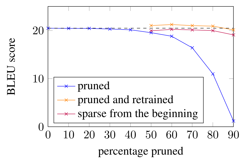
Figure 8: src
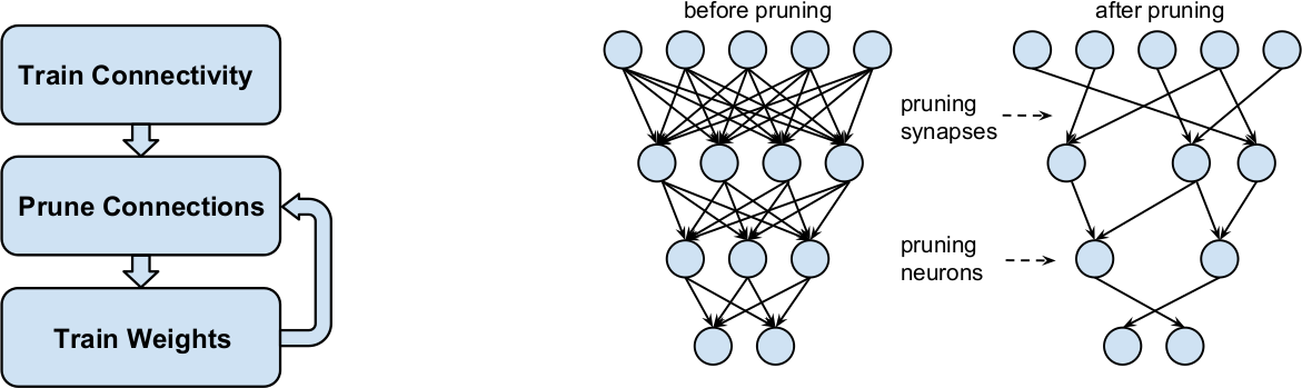
Figure 9: Learning both Weights and Connections for Efficient Neural Network, (2015)
There are many different methods for pruning, e.g. magnitude (unstructured) pruning and structured pruning. Which is best suited depends on the hardware the model will be deployed on.
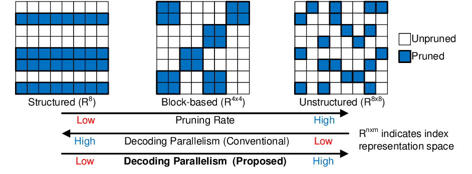
Figure 10: src
3.1. Magnitude pruning (Unstructured pruning):
Also known as Unstructured pruning, convert all weights below a threshold to zero. This reduces storage requirements.
- Pick a pruning factor X
- In each layer, set lowest X % of weights, by absolute value, to 0
- Optional: retrain model to recover accuracy
Similarly, during training, we can use L1 or L2 regularization to penalize non-zero weights.
Note: In order to actually get an improvement in computational resources, one must use a sparse execution engine, that makes use of the sparsity of the weight matrix.
Storing and computing (unstructured) matrix with zeros takes same amount of time, unless we convert the matrix to some sparse representation, e.g. Sparse MatMul.
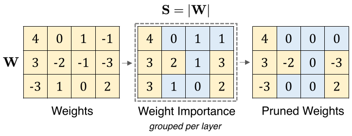
Figure 11: [src]
3.2. Structured pruning:
Enforce a structured pattern in the network on which weights are allowed to be zeroed out. Thus we remove entire layers or components from the model, that can directly lead to computational speed up.
Consider a N:M structured sparsity pattern:
- For each block of M consecutive values in a matrix (row), only N are allowed to be non-zero
- Only store the values we keep (don’t store zero elements)
Can be done with either:
- One-shot pruning
- Prunes fully-trained network
- Iterative pruning
- Prune network gradually
Benefit:
- Good for Nvidia Tensor Core efficiency
3.3. SparseGPT
In the paper SparseGPT: Massive Language Models Can Be Accurately Pruned in One-Shot (arXiv) they introduced a pruning method tailored for GPT LLM-models but also works with other models.
We show for the first time that large-scale generative pretrained transformer (GPT) family models can be pruned to at least 50% sparsity in one-shot, without any retraining, at minimal loss of accuracy.
- Can achieve 50% pruning, while magnitude pruning can only reach 10% before performance hit.
- No retraining
- Layer by layer pruning, then stitched together in the end
- Requires expensive weight update process, (inversion of second-order Hessian matrix)
3.4. Wanda - (Pruning by Weights AND Activations)
- No weight updates
- No retraining
Wanda: Prune weights based on magnitude and input activation:
- Prune weights by magnitude and input activations
Done by:
- Pruning metric - how to compare the Weights
- Pruning granularity - which weights to compare
- set sparsity level, e.g. 50%, removing half of all weights on each row, determined by size of weight x input activations
- repeat for each hidden layer
- input activations determined by calibration data set
- does not need to update weights after pruning, unlike structured pruning
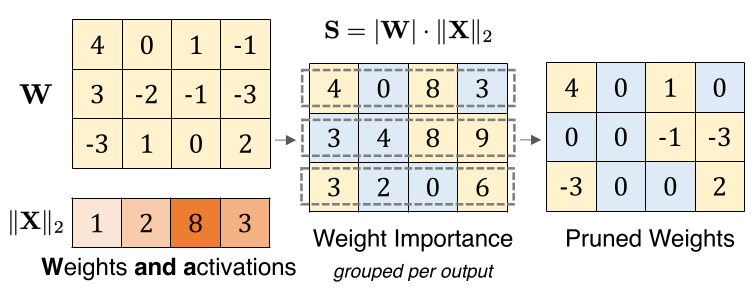
Figure 12: [src]
| Weight update | Calibraiton data | LLaMA 7B | LLaMA 65B | LLaMA 7B | LLaMA 65B | |
|---|---|---|---|---|---|---|
| (Perplex) | Perplex) | (speed) | (speed) | |||
| Magnitude | No | No | ||||
| SparseGPT | Yes | Yes | 7.22 | 3.98 | 203 s | 1354 s |
| Wanda | No | Yes | 7.26 | 3.98 | 0.54 s | 5.6 s |
4. Knowledge distillation (model distillation)
If we can extract the knowledge from the data it is quite easy to distill most of it into a much smaller model for deployment.
Geoffrey Hinton (slides)
We can reduce the size and complexity of a model by “distilling” the knowledge of the first “teacher model”, down to a smaller “student model” that still preserves the performance, by mimicking the teacher.
Consider classification, where the (teacher) model learns probability distribution of each possible label. We can train a smaller and simpler “student” network to yield the same probability distribution as the teacher, given the same input. It will be faster to train as it has more input (full probability distribution of each label, for each input to classify), than the teacher network which only had binary input from the labels.
- train teacher network.
- train student network to predict output of teacher
E.g. if classification, input to teacher is just labels, while student input is probability distribution (from the output of the teacher), i.e. more information to learn.
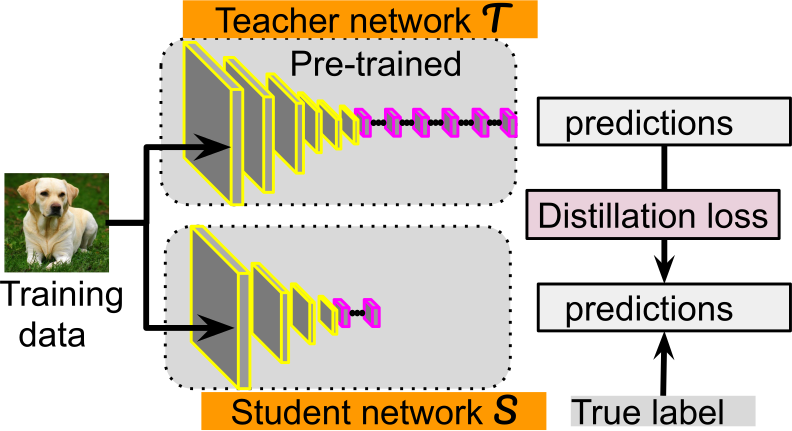
Figure 13: src
Example: DestilBERT (BERT is teacher), the student had 40% of the weights, yet maintained 97% of the accuracy.)
                                 soft
                  +---------+    labels
+--------+   +--> | TEACHER |-------------+
|     {s}|   |    +---------+             |
|        | x |                   soft     +--> +-------------------+
|  DATA  +---+                   predictions   | KL Divergence {io}| --> distillation
|        |   |                 +-------------> | cGRE              |     loss
|cPNK    |   |    +---------+  |               +-------------------+
+--------+   +--> | STUDENT |--+ hard
    |             +---------+  | predictions   +-------------------+
    |                          +-------------> | Cross Entropy {io}| --> student
    |      y     Ground truth                  | cGRE              |     loss
    +----------------------------------------> +-------------------+
                                 hard labels
Student model could have different architecture like fewer layers - biggest potential gain in speed, compared to pruning / quantization, however it is still computationally heavy.
In Born-Again Neural Networks (2018), they trained a model using itself as the teacher (same parameterization), and still saw students outperform the teacher.
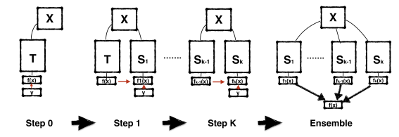
Figure 14: Teacher trained using labels Y, to yield prediction X used for Student. src
5. Engineering / hardware integration
6. Appendix
Network Trimming: A Data-Driven Neuron Pruning Approach towards Efficient Deep Architectures, 2016 (arXiv)
we introduce network trimming which iteratively optimizes the network by pruning unimportant neurons based on analysis of their outputs on a large dataset. Our algorithm is inspired by an observation that the outputs of a significant portion of neurons in a large network are mostly zero, regardless of what inputs the network received.
Self-Compressing Neural Networks, 2023 (arXiv)
We propose Self-Compression: a simple, gen- eral method that simultaneously achieves two goals: (1) re- moving redundant weights, and (2) reducing the number of bits required to represent the remaining weights […] In our experiments we demonstrate floating point accuracy with as few as 3% of the bits and 18% of the weights remaining in the network.
Learning Efficient Convolutional Networks through Network Slimming, 2017 (arXiv)
[reduced model size and footprint is] achieved by enforcing channel-level sparsity in the network in a simple but effective way. Different from many existing approaches, the proposed method directly applies to modern CNN 3architectures […] We call our approach network slimming, which takes wide and large networks as input models, but during training insignificant channels are automatically identified and pruned afterwards, yielding thin and compact models with comparable accuracy.
Learning both Weights and Connections for Efficient Neural Networks, 2015 (arXiv)
conventional networks fix the architecture before training starts; as a result, training cannot improve the architecture. To address these limitations, we describe a method to reduce the storage and computation required by neural networks by an order of magnitude without affecting their accuracy by learning only the important connections. Our method prunes redundant connections using a three-step method. First, we train the network to learn which connections are important. Next, we prune the unimportant connections. Finally, we retrain the network to fine tune the weights of the remaining connections.
Distilling the Knowledge in a Neural Network, 2015 (arXiv)
[it’s been] shown that it is possible to compress the knowledge in an ensemble into a single model which is much easier to deploy and we develop this approach further using a different compression technique. We achieve some surprising results on MNIST and we show that we can significantly improve the acoustic model of a heavily used commercial system by distilling the knowledge in an ensemble of models into a single model. […] Unlike a mixture of experts, these specialist models can be trained rapidly and in parallel.
- Knowledge Distillation and Student-Teacher Learning for Visual Intelligence: A Review and New Outlooks, 2021 (arXiv)
- Distiller - an open-source Python package for neural network compression research.
- Integer Quantization for Deep Learning Inference: Principles and Empirical Evaluation, 2020 (arXiv)
- Deep Compression: Compressing Deep Neural Networks with Pruning, Trained Quantization and Huffman Coding, 2015 (arXiv)
- A Simple and Effective Pruning Approach for Large Language Models, 2023 (arXiv)
- Compression of Neural Machine Translation Models via Pruning, 2016 (arXiv)
- Course on LLM including fine tuning and quantization llm-course