
Conserving memory when reading SQL tables in python pandas
Published on Apr 22, 2021 by Impaktor.
For surely the food that memory gives to eat is bitter to the taste, and it
is only with the teeth of hope that we can bear to bite it.
“She”, H. Rider Haggard
1. Introduction
Herein, I will outline the several “gotchas” I have stumbled upon in my quest to read data from an SQL table using python pandas in a memory efficient way. In my case, the table was 52M rows, 23 columns, and used 900 MB RAM when loaded, but uses north of 12 GB when fetching it from SQL, which was more than the production environment ideally can handle. In this post I detail different solutions that each will reduce memory consumption.
Below is the first generic starting code which I want to improve. All other snippets are additions/modifications of the below code. (It is assumed you have a working connection to SQL from python from before. Here, we use luigi to read in needed parameters.)
import pandas as pd
import pyodbc

# We use luigi to get the SQL user, password, database, and driver.
# It's assumed you can conjure up correct information to establish a
# pyodbc connection to SQL
import luigi

def get_db():
    """Returns connection object to SQL"""
    config = luigi.configuration.get_config()
    kwargs = dict(config.items("database"))
    return pyodbc.connect(**kwargs)

# Table name to be read
table = "my_table"

# Get connection to SQL database
conn = get_db()

# Select only the columns we actually need, from SQL
columns = ["COLUMN01",
           "COLUMN02",
           # ....
           "COLUMN23"]

query = f"""SELECT {', '.join(columns)} FROM {table}"""

df = pd.read_sql(query, conn).reset_index(drop=True)
Since the end goal is to run this in a docker image in production environment, we do all bench marking, such as RAM usage, by monitoring the running docker image, as described in a previous post. We see it reaches 12 GB of RAM use in the figure below (we sample the RAM usage once per second). For interest, we also include CPU usage.
After all the data is loaded from SQL, it is validated using Great Expectations, which is the second half of activity seen below. When this is done, it returns, and the docker image stops, which here takes under 2 minutes.
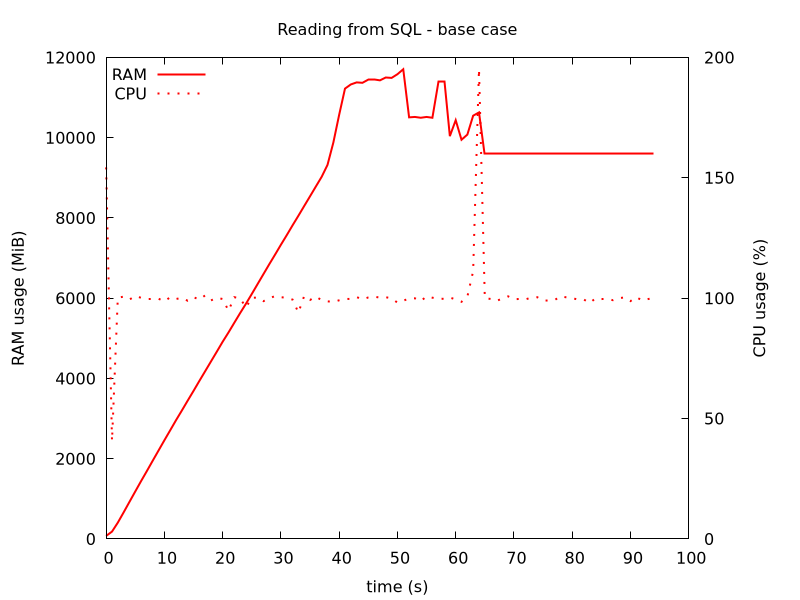
Figure 1: Our starting base case. RAM usage hits 12 GB
2. Improvement 1: Read SQL database in chunks
Pandas’ read_sql() has an argument chunksize, if given it will return the
data in chunks. We will then have to concatenate each df, corresponding to
the chunks.
Since we are appending, we need to initialize a data frame, and specify the columns.
df = pd.DataFrame(columns=columns)

chunksize = 100_000
for i, df_chunk in enumerate(pd.read_sql(query, conn, chunksize=chunksize)):
    df = pd.concat((df, df_chunk), axis=0, copy=False)
    print(f"{i} Got dataframe with {len(df_chunk):,} rows")

df = df.reset_index(drop=True)
With this modification, RAM usage goes down and now peaks at 8 GB. But this is not one 50th of what we had when we read in all 52M rows at once, why?
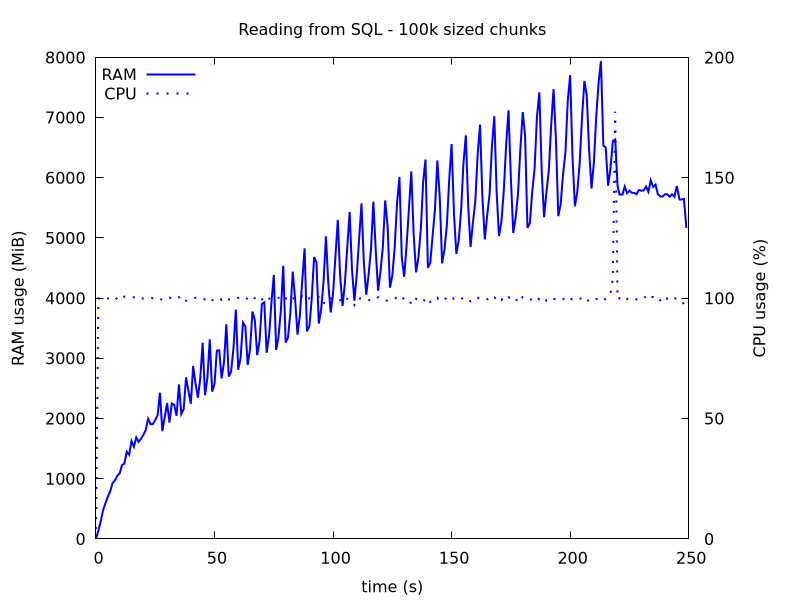
Figure 2: Reading SQL in chunks of size 100k.
3. Improvement 2: Read SQL database in chunks (properly!)
It turns out, when setting chunksize, it just returns it in chunks, it still reads and loads the table all at once, as detailed in this blog post.
This is fixed by using sqlalchemy, instead of pyodbc to establish a
connection, and setting stream_results=True (there is an open issue on
pandas to do this by default).
from sqlalchemy import create_engine
import luigi

def get_db():
    """Returns connection object to SQL"""
    config = luigi.configuration.get_config()
    kwargs = dict(config.items("database"))

    engine_stmt = ("mssql+pyodbc://%s:%s@%s/%s?driver=%s" % \
                   (kwargs['uid'],
                    kwargs['pwd'],
                    kwargs['server'],
                    kwargs['database'],
                    kwargs['driver'])) # 'ODBC+DRIVER+17+for+SQL+Server'

    # Query in streaming chunk size, to save RAM.
    engine = create_engine(engine_stmt)
    conn = engine.connect().execution_options(stream_results=True)
    return conn
However, this did not get me below 6GB of RAM usage (results not shown).
4. Improvement 3: Make ’category’ columns work with concatenate
Depending on the data, significant RAM can be saved by casting each column into more suitable data types, especially if few values are repeated often, such that we can cast to category type. However, since we are concatenating the chunked reading, the “top”/original df and the “bottom”/appending one need to be in agreement with which categories map, internally, to which placeholder index, which we now address here.
4.1. Strategy to find best dtype for each column
Columns with few integers need not be represented as the default
np.int64. E.g. a persons “age”, is a number between 0-127, thus
np.int8, or np.uint8, is enough to represent numbers in the interval
[-127, 127] or [0, 255], respectively. Similarly for bool, datetime64,
etc.
For columns of object type, consisting of only a few unique repeated values, the best representation is as category type, such that they are internally represented by an index + lookup dictionary.
Use df.info() to see full ram usage of the data frame, and
df.memory_usage(deep=True, index=False) to break it down on each column,
and combine with df.nunique().
Below is a function I wrote to serve this purpose, that returns a df with needed information to make a decision.
def mem_usage(df):
    """Display each column's memory usage, dtype, and number of unique values,
    e.g. for assessing optimal data type for each column.

    Parameters
    ----------
    df : pd.DataFrame
        A pandas data frame, with data to be probed

    Returns
    -------
    pd.DataFrame
        Data frame summarizing the stas of input df.
    """
    mem = df.memory_usage(deep=True, index=False).rename('mem')
    typ = df.dtypes.rename('dtype')
    unq = df.nunique().rename('nunique')
    nan = df.isna().sum().rename('Nans')

    # If N < classes, get relative value count distribution:
    N_class = 5
    stat = pd.Series(index=mem.index, dtype=str).fillna("-").rename('stats')
    for col in unq[unq < N_class].index:
        v = df[col].value_counts() / len(df)
        print(col)
        stat[col] = ", ".join([f"{i:.2}" for i in v])

    print(f"Total memory usage: {mem.sum()/1000**2:,.2f} MB")
    return pd.concat([mem, typ, unq, nan, stat], axis=1)
4.2. Applying on our example data
The table below shows a diagnosis of our 52M x 23 data frame. We see that much of the size originates from COLUMN07 - COLUMN11, which are all just repetitions of a few unique values (10, or 31) making them prime candidates for categorical type. Similar for other columns, e.g. the last two.
| Title | Unique | Size | dtypes |
|---|---|---|---|
| COLUMN01 | 5252294 | 627963342 | object |
| COLUMN02 | 21123 | 421612999 | object |
| COLUMN03 | 383098 | 429001287 | object |
| COLUMN04 | 9407 | 54018352 | datetime64[ns] |
| COLUMN05 | 834 | 54018352 | float64 |
| COLUMN06 | 51882 | 54018352 | float64 |
| COLUMN07 | 174 | 422764016 | object |
| COLUMN08 | 10 | 390175396 | object |
| COLUMN09 | 10 | 459187154 | object |
| COLUMN10 | 31 | 396693120 | object |
| COLUMN11 | 31 | 445256806 | object |
| COLUMN12 | 8101 | 54018352 | float64 |
| COLUMN13 | 11607 | 54018352 | float64 |
| COLUMN14 | 6081 | 54018352 | float64 |
| COLUMN15 | 5392 | 54018352 | datetime64[ns] |
| COLUMN16 | 4851 | 54018352 | datetime64[ns] |
| COLUMN17 | 1411 | 54018352 | float64 |
| COLUMN18 | 712 | 627950508 | object |
| COLUMN19 | 712 | 422654617 | object |
| COLUMN20 | 22 | 54018352 | float64 |
| COLUMN21 | 2 | 54018352 | float64 |
| COLUMN22 | 3 | 464442564 | object |
| COLUMN23 | 5 | 445651704 | object |
4.3. Reading from SQL and concatenating categorical data frames
The main caveat when concatenating categorical columns, is that we must also combine the underlying lookup dictionary between the known categories (which is different between different data frames), as a category that is only represented in the new appending df will not exist in the original df’s looup dictionary. Below demonstrates how to fix this:
from pandas.api.types import union_categoricals

# Example of columns that should be cast to categorical type
categorical = ["COLUMN07", "COLUMN08", "COLUMN22", "COLUMN23"]

df = pd.DataFrame(columns=columns).astype({col: 'category' for col in categorical})

chunksize = 100_000
for i, df_chunk in enumerate(pd.read_sql(query, conn, chunksize=chunksize)):

     # Cast to categorical, and prepare df for concatenation
     df_chunk = df_chunk.astype({col: 'category' for col in categorical})
     for col in categorical:
         uc = union_categoricals([df[col], df_chunk[col]])
         df[col] = pd.Categorical(df[col], categories=uc.categories)
         df_chunk[col] = pd.Categorical(df_chunk[col], categories=uc.categories)

     df = pd.concat((df, df_chunk), axis=0, copy=False)
     print(f"{i} Got dataframe with {len(df_chunk):,} rows")
df = df.reset_index(drop=True)
This code reduces RAM usage to below 5 GB, for our data.
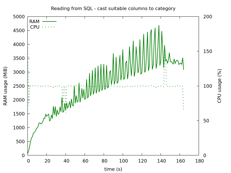
Figure 3: Reading SQL in chunks of size 100k, and casting 7 columns to category type, before concatenating
5. Improvement 4: Avoid using pandas concatenate!
It turns out that the real offending culprit is pd.concat(), which uses
multiple times more RAM than the resulting df. The workaround is to not use
it, e.g. by concatenating manually to disk, instead of to RAM, as
pd.concat does. This is addressed in this post where they use
read_csv(), but since we are reading from sql, we use the code snippet
below.
Note: when incrementally fetching data with an OFFSET, it is important the column we are telling SQL to do its ordering on is all unique values, or there will be repeating rows, from the different chunks.
import pyarrow
import pyarrow.parquet as pq

chunksize, chunk = 100_000, 0

# Note: values in ordering column (here: 'COLUMN01') must be all unique:
q = query + " ORDER BY COLUMN01 OFFSET {} ROWS FETCH NEXT {} ROWS ONLY"

while True:
    df_tmp = pd.read_sql_query(q.format(chunksize*chunk, chunksize), conn)

    # Save df to parquet by appending
    table = pyarrow.Table.from_pandas(df_tmp)
    pq.write_to_dataset(table, root_path="disk_data", use_deprecated_int96_timestamps=True)

    print(f"Got chunk {chunk} of size {len(df_tmp):,}")

    if len(df_tmp) < chunksize:
        break
    chunk += 1

df = pd.read_parquet("disk_data").reset_index(drop=True)
Note, "disk_data" here is the name of a folder. One can wrap the block in
a with tempfile.TemporaryDirectory() as disk_data block.
This used 500 MiB RAM during reading from SQL, and then a spike just below 4 GB when reading the data back, and validating it using Great Expectations, as mentioned in the 1.
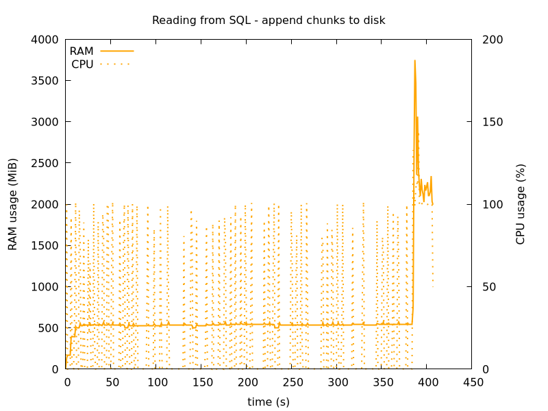
Figure 4: Reading SQL in chunks of size 100k, and appending to disk.
6. Conclusion
Comparing all methods together, its more clear that there is also a trade off with speed. Appending to disk is the slowest, but saves the most memory usage. The increase in RAM towards the end is due to Great Expectations reading in the full data and running validations on it.
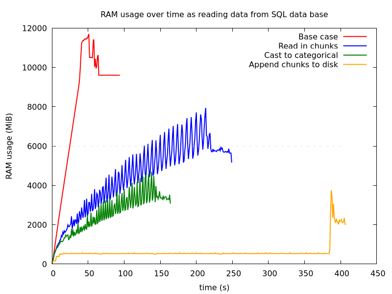
Figure 5: Reading SQL data from SQL - comparison