PyTorch from first principles
Published on Sep 18, 2020 by Impaktor.
- Spock: A computer can process information but only the information which
is put into it
- Kirk: Granted it can work a thousand, a million times faster than the
human brain but it cant make a valued decision it has no intuition
it cant think.
Star Trek “The Ultimate Computer”, TOS
Table of Contents
- 1. Introduction
- 2. Data generation
- 3. Split data into train/test numpy
- 4. Intermission 1: General pointers on tensors pytorch
- 5. Data to tensors pytorch
- 6. Tensor for data != tensor for parameters pytorch
- 7. Intermission 2: Gradient descent optimization, in 5 steps numpy
- 8. Autograd, your companion for all your gradient needs! pytorch
- 9. Dynamic Computation Graph: what is that? pytorch
- 10. Optimizer: learning the parameters step-by-step pytorch
- 11. Loss: aggregating erros into a single value pytorch
- 12. Model: making predictions pytorch
- 13. Dataset dataset
- 14. DataLoader, splitting your data into mini-batches
- 15. Evaluation: does it generalize?
- 16. Training Loop
- 17. Final Code
- 18. BONUS: Further Improvements
- 19. Appendix 0: Some overview
- 20. Appendix A: Further
- 21. Appendix B: Autoencoder
- 22. TODO Appendix C: Monitoring & Logging
1. Introduction
PyTorch, quickly gaining popularity, and is becoming the default framework for new implementations, e.g. the Transformer library. This it the tutorial I worked through to get started. It is mostly a copy-paste from PyTorch101_ODSC_London2019 (by David Voigt Godoy github), with some re-writes, additions, clarifications, and additions, written for my own use, and two appendices added (mostly for my own enjoyment). There are other resources, perhaps additionally looking into this post on PyTorch internals.
Rather than demonstrating PyTorch by doing a classic image classification, we’ll focus on a linear regression, with a single feature \(x\), to not distracts from the main goal: how does PyTorch work?. Specifically:
\begin{equation} y = a + b x + \epsilon \end{equation}2. Data generation
import numpy as np
import matplotlib.pyplot as plt
# %matplotlib inline
plt.style.use('fivethirtyeight')

import torch
import torch.optim as optim
import torch.nn as nn
from torchviz import make_dot

true_a = 1
true_b = 2
N = 100

# Data Generation
np.random.seed(42)
x = np.random.rand(N, 1)
y = true_a + true_b * x + .1 * np.random.randn(N, 1)
3. Split data into train/test numpy
Next, let’s split our synthetic data into train and validation sets, shuffling the array of indices and using the first 80% shuffled points for training. Following is how we can do it with numpy:
# Shuffles the indices
idx = np.arange(N)
np.random.shuffle(idx)

# Use first 80% random indices for train
train_idx = idx[:int(N*.8)]
# Use remaining indices for validation
val_idx = idx[int(N*.8):]

# Generate train and validation sets
x_train, y_train = x[train_idx], y[train_idx]
x_val, y_val = x[val_idx], y[val_idx]

# PLOT DATA
# ---------
fig, ax = plt.subplots(1, 2, figsize=(12, 4))
ax[0].scatter(x_train, y_train)
ax[0].set_xlabel('x')
ax[0].set_ylabel('y')
ax[0].set_ylim([1, 3])
ax[0].set_title('Generated Data - Train')
ax[1].scatter(x_val, y_val, c='r')
ax[1].set_xlabel('x')
ax[1].set_ylabel('y')
ax[1].set_ylim([1, 3])
ax[1].set_title('Generated Data - Validation')
fig.savefig("/tmp/train_and_validation_data.png", bbox_inches="tight")
4. Intermission 1: General pointers on tensors pytorch
In Numpy, you may have an array that has three dimensions. That is, technically speaking, a tensor.
A scalar (a single number) has zero dimensions, a vector has one dimension, a matrix has two dimensions and a tensor has three or more dimensions.
But, to keep things simple, it is commonplace to call vectors and matrices tensors as well — so, from now on, everything is either a scalar or a tensor.
(For a discussion on anatomy of all the different tensor computation libraries, and what the differences between them are, see: https://eigenfoo.xyz/tensor-computation-libraries/)
You can create tensors in PyTorch pretty much the same way you create arrays in Numpy. Using tensor() you can create either a scalar or a tensor.
PyTorch’s tensors have equivalent functions as its Numpy counterparts, like: ones(), zeros(), rand(), randn() and many more.
Creating tensors:
- eye creates diagonal matrix / tensor
- zeros creates tensor filled with zeros
- ones creates tensor filled with ones
- linspace creates linearly increasing values
- arange linearly increasing integers
Examples of generating torch tensors:
BIG caveat: .reshape() and .view() create a new tensor with the
desired shape that shares the underlying data with the original
tensor! -> Use copy() or clone() first.
scalar = torch.tensor(3.14159)
vector = torch.tensor([1, 2, 3])
matrix = torch.ones((2, 3), dtype=torch.float)
tensor = torch.randn((2, 3, 4), dtype=torch.float)
for obj in [scalar, vector, matrix, tensor]:
    print(f"\n{obj.size()}, {obj.shape}")
    print(obj)
I.e. some operations share underlying memory, some create new tensors:
- Copy Data
- type casting
torch.Tensor()torch.tensor()torch.clone()
- Share Data
torch.as_tensor()torch.from_numpy()torch.view()torch.reshape()
Generally on matrices/tensors in Torch:
# An un-initialized matix contains what happend to be in that memory address
print(torch.empty(5, 3))

# random floats [0,1]
a = torch.rand(5, 3)

# standard numpy indexing with all bells and whistles
print(a[:, 1])

# matrix filled zeros, of dtype long
b = torch.zeros(5, 3, dtype=torch.long)
print(torch.add(a, b))

# ...or supply output tensor as argument
result = torch.empty(5, 3)
torch.add(a, b, out=result)
print(result)

# adds b to a, in-place
a.add_(b)
print(a)

# resize using torch.view
a = torch.randn(4, 4)
b = a.view(16)
c = a.view(-1, 8)  # the size -1 is inferred from other dimensions
print(a.size(), b.size(), c.size())
As we’ll see, any method suffixed with .method_() is an in-place
operation.
5. Data to tensors pytorch
Let’s return to our linear regression problem from that excursion on tensors.
Data is stored in tensors, either on CPU or GPU memory. The from_numpy() returns a tensor, although it’s on the CPU. We can use to() to put it on the GPU.
# Our data was in Numpy arrays, but we need to transform them into PyTorch's Tensors
# (Also cast to lower 32 bit precision)
x_train_tensor = torch.from_numpy(x_train).float()
y_train_tensor = torch.from_numpy(y_train).float()

# Put data on GPU if available, and use that tensor instead!
device = 'cuda' if torch.cuda.is_available() else 'cpu'
x_train_tensor = x_train_tensor.to(device)
y_train_tensor = y_train_tensor.to(device)

# First is numpy array, second being torch tensor
print(f"python type():\t {type(x_train)}, {type(x_train_tensor)}")

# Use pytorch's type()-method to see where data is:
print(f"pytorch type():\t {x_train_tensor.type()}")

# To convert back to numpy, but must first move GPU -> CPU
# x_train_tensor.cpu().numpy()
6. Tensor for data != tensor for parameters pytorch
torch.Tensor is the central class of the package. If you set its attribute
.requires_grad as True, it starts to track all operations on it. We
shall see that when one finishes computations, one can call .backward()
and have all the gradients computed automatically. The gradient for this
tensor will be accumulated into .grad attribute.
# Unlike a tensor for data, a tensor for a learnable parameter requires
# gradient! thus, must pass: requires_grad=True

# Assign tensors to a device at creation time, to avoid problems:
a = torch.randn(1, requires_grad=True, dtype=torch.float, device=device)
b = torch.randn(1, requires_grad=True, dtype=torch.float, device=device)
print(a, b)
7. Intermission 2: Gradient descent optimization, in 5 steps numpy
Before diving into our solution PyTorch, it’s very instructive to first do a gradient decent in pure numpy, even if you know this, make sure to skim through it, and understand the code, as this defined the structure we’ll model everything else on later.
- Random initialize parameters / weights
- Compute model’s predictions — forward pass
- Compute loss
- Compute the gradients
- Update the parameters
- Rinse and repeat!
For more:
7.1. Step 0. Random initialization
Must initialize our parameters (a, b), (using just numpy)
np.random.seed(42)
a = np.random.randn(1)
b = np.random.randn(1)
print(a, b)
7.2. Step 1. Compute predictions — forward pass
7.3. Step 2. Compute Loss
- Error
Difference between actual and predicted value for single data point
\begin{equation} \text{error}_i = (y_i - \hat{y}_i) \end{equation}- Loss
Aggregate of errors, for regression typically MSE
\begin{equation} \text{MSE} = \frac{1}{N} \sum_i^N \text{error}_i^2 = \frac{1}{N} \sum_i^N (y_i - \hat{y}_i)^2 \end{equation}
It is worth mentioning that, if we compute the loss using:
- All points in the training set (N), we are performing a batch gradient descent
- A single point at each time, it would be a stochastic gradient descent
- Anything else (n) in-between 1 and N characterizes a mini-batch gradient descent
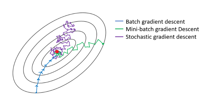
Figure 1: Gradient descent batching
# How wrong is our model? That's the error!
error = (y_train - yhat)

# It is a regression, so it computes mean squared error (MSE)
loss = (error ** 2).mean()
print(f"loss: {loss}")
7.4. Step 3. Compute the Gradients
A gradient is a partial derivative — why partial? Because one computes it with respect to (w.r.t.) a single parameter. We have two parameters, \(a\) and \(b\), so we must compute two partial derivatives.
A derivative tells you how much a given quantity changes when you slightly vary some other quantity. In our case, how much does our MSE loss change when we vary each one of our two parameters?
The right-most part of the equations below is what you usually see in implementations of gradient descent for a simple linear regression. The intermediate steps show all elements that pop-up from the application of the chain rule.
The gradient is how much the loss changes if one parameter changes a little bit.
Taking the partial derivative for w.r.t \(a\) and \(b\) yields:
\begin{equation*} \large \frac{\partial{\text{MSE}}}{\partial{a}} = \frac{\partial{\text{MSE}}}{\partial{\hat{y_i}}} \cdot \frac{\partial{\hat{y_i}}}{\partial{a}} = \frac{1}{N} \sum_{i=1}^N{2(y_i - a - b x_i) \cdot (-1)} = -2 \frac{1}{N} \sum_{i=1}^N{(y_i - \hat{y_i})} \end{equation*} \begin{equation*} \large \frac{\partial{\text{MSE}}}{\partial{b}} = \frac{\partial{\text{MSE}}}{\partial{\hat{y_i}}} \cdot \frac{\partial{\hat{y_i}}}{\partial{b}} = \frac{1}{N} \sum_{i=1}^N{2(y_i - a - b x_i) \cdot (-x_i)} = -2 \frac{1}{N} \sum_{i=1}^N{x_i (y_i - \hat{y_i})} \end{equation*}# Computes gradients for both "a" and "b" parameters a_grad = -2 * error.mean() b_grad = -2 * (x_train * error).mean() print(a_grad, b_grad)
7.5. Step 4. Update the Parameters
In the final step, we use the gradients to update the parameters. Since we are trying to minimize our losses, we reverse the sign of the gradient for the update.
There is still another parameter to consider: the learning rate, denoted by the Greek letter eta (\(\eta\)), which is the multiplicative factor that we need to apply to the gradient for the parameter update.
\begin{equation*} \large a = a - \eta \frac{\partial{\text{MSE}}}{\partial{a}} \end{equation*} \begin{equation*} \large b = b - \eta \frac{\partial{\text{MSE}}}{\partial{b}} \end{equation*}Let’s start with a value of 0.1 (which is a relatively big value, as far as learning rates are concerned!).
The learning rate is the single most important hyper-parameter to tune when you are using Deep Learning models!
# Sets learning rate
lr = 1e-1

# Updates parameters using gradients and the learning rate
print(a, b)
a = a - lr * a_grad
b = b - lr * b_grad

print(a, b)
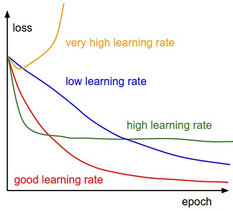
Figure 2: Learning rates matter
7.6. Step 5. Rinse and Repeat!
Now we use the updated parameters to go back to step 1 and restart the process.
Repeating this process over and over, for many epochs, is, in a nutshell, training a model.
An epoch is complete whenever every and all \(N\) points have been used once for computing the loss:
- batch gradient descent
- trivial: it uses all points for computing the loss - one epoch is the same as one update
- stochastic gradient descent
- one epoch means N updates
- mini-batch (of size n)
- one epoch has N/n updates
Let’s put the previous pieces of code together and loop over many epochs:
(Keep in mind that, if you don’t use batch gradient descent (below), you’ll have to write an inner loop to perform the five training steps for either each individual point (stochastic) or \(n\) points (mini-batch). We’ll see a mini-batch example later down the line.)
# Define number of epochs
n_epochs = 1000

# Step 0
np.random.seed(42)
a = np.random.randn(1)
b = np.random.randn(1)

for epoch in range(n_epochs):
    # Step 1:
    # Compute our model's predicted output
    yhat = a + b * x_train

    # Step 2:
    # How wrong is our model? That's the error!
    error = (y_train - yhat)
    # It is a regression, so it computes mean squared error (MSE)
    loss = (error ** 2).mean()

    # Step 3:
    # Compute gradients for both "a" and "b" parameters
    a_grad = -2 * error.mean()
    b_grad = -2 * (x_train * error).mean()

    # Step 4:
    # Update parameters using gradients and the learning rate
    a -= lr * a_grad
    b -= lr * b_grad
print(a, b)
Sanity check:
# Sanity Check: do we get the same results as our gradient descent?
from sklearn.linear_model import LinearRegression
linr = LinearRegression()
linr.fit(x_train, y_train)
print(linr.intercept_, linr.coef_[0])
Now this was done in numpy, let’s do it in pytorch!
8. Autograd, your companion for all your gradient needs! pytorch
Autograd is PyTorch’s automatic differentiation package. Thanks to it, we don’t need to worry about partial derivatives, chain rule or anything like it. (Also, see “Autograd Explained - In-depth Tutorial” in 13 min, youtube).
The autograd package provides automatic differentiation for all operations on Tensors. It is a define-by-run framework, which means that the backprop is defined by how the code is run, and that every single iteration can be different.
So, how do we tell PyTorch to do its thing and compute all gradients? That’s
what backward() is good for.
Recall, that the starting point for computing the gradients was the loss, as
we computed its partial derivatives w.r.t. our parameters. Hence, we need to
invoke the backward() method from the corresponding Python variable, like,
loss.backward().
8.1. Backward
# Step 0
torch.manual_seed(42)

a = torch.randn(1, requires_grad=True, dtype=torch.float, device=device)
b = torch.randn(1, requires_grad=True, dtype=torch.float, device=device)

# Step 1
# Compute our model's predicted output
yhat = a + b * x_train_tensor

# Step 2
# How wrong is our model? That's the error!
error = (y_train_tensor - yhat)
# It is a regression, so it computes mean squared error (MSE)
loss = (error ** 2).mean()

# Step 3
# No more manual computation of gradients!
loss.backward()

# Computes gradients for both "a" and "b" parameters
# a_grad = -2 * error.mean()
# b_grad = -2 * (x_train_tensor * error).mean()
8.2. grad / zero_
What about the actual values of the gradients? We can inspect them by looking at the grad attribute of a tensor.
print(f"Pytorch gradient: {a.grad}, {b.grad}")
So, every time we use the gradients to update the parameters, we need to
zero the gradients afterwards. And that’s what zero_() is good for.
In PyTorch, every method that ends with an underscore (_) makes changes in-place, meaning, they will modify the underlying variable.
a.grad.zero_(), b.grad.zero_()
So, let’s ditch the manual computation of gradients and use both backward()
and zero_() methods instead.
We are still missing Step 4, that is, updating the parameters. Let’s include it as well…
# Step 0
torch.manual_seed(42)
a = torch.randn(1, requires_grad=True, dtype=torch.float, device=device)
b = torch.randn(1, requires_grad=True, dtype=torch.float, device=device)

# Step 1
# Compute our model's predicted output
yhat = a + b * x_train_tensor

# Step 2
# How wrong is our model? That's the error!
error = (y_train_tensor - yhat)
# It is a regression, so it computes mean squared error (MSE)
loss = (error ** 2).mean()

# Step 3
# No more manual computation of gradients!
loss.backward()
# Computes gradients for both "a" and "b" parameters
# a_grad = -2 * error.mean()
# b_grad = -2 * (x_train_tensor * error).mean()
print(a.grad, b.grad)

# Step 4
# Update parameters using gradients and the learning rate
with torch.no_grad(): # what is that?!
    a -= lr * a.grad
    b -= lr * b.grad

# PyTorch is "clingy" to its computed gradients, we need to tell it to let it go...
a.grad.zero_()
b.grad.zero_()

print(a.grad, b.grad)
8.3. no_grad()
One does not simply update parameters without no_grad
Why do we need to use no_grad() to update the parameters?
The culprit is PyTorch’s ability to build a dynamic computation graph from every Python operation that involves any gradient-computing tensor or its dependencies (this is useful for RNNs).
What is a dynamic computation graph?
Don’t worry, we’ll go deeper into the inner workings of the dynamic computation graph in the next section.
So, how do we tell PyTorch to “back off” and let us update our parameters without messing up with its fancy dynamic computation graph?
That is the purpose of no_grad(): it allows us to perform regular Python
operations on tensors, independent of PyTorch’s computation graph. Torch
will thus stop tracking gradients for any tensor wrapped in no_grad or,
alternatively, by applying a .detatch() method on the tensor.
lr = 1e-1
n_epochs = 1000

# Step 0
torch.manual_seed(42)
a = torch.randn(1, requires_grad=True, dtype=torch.float, device=device)
b = torch.randn(1, requires_grad=True, dtype=torch.float, device=device)

for epoch in range(n_epochs):
    # Step 1
    # Compute our model's predicted output
    yhat = a + b * x_train_tensor

    # Step 2
    # How wrong is our model? That's the error!
    error = (y_train_tensor - yhat)
    # It is a regression, so it computes mean squared error (MSE)
    loss = (error ** 2).mean()

    # Step 3
    # No more manual computation of gradients!
    loss.backward()

    # Step 4
    # Update parameters using gradients and the learning rate
    with torch.no_grad():
        a -= lr * a.grad
        b -= lr * b.grad

    # PyTorch is "clingy" to its computed gradients, we need to tell it to let it go...
    a.grad.zero_()
    b.grad.zero_()

print(a, b)
Finally, we managed to successfully run our model and get the resulting parameters. Surely enough, they match the ones we got in our Numpy-only implementation.
Let’s take a look at the loss at the end of the training…
print("loss", loss)
What if we wanted to have it as a Numpy array? I guess we could just use
numpy() again, right? (and cpu() as well, since our loss is in the cuda
device… No, because unlike our data tensors, the loss tensor is actually
computing gradients - and in order to use numpy, we need to detach() that
tensor from the computation graph first:
loss.detach().cpu().numpy()
This seems like a lot of work, there must be an easier way! And there is
one indeed: we can use item(), for tensors with a single element or
tolist() otherwise.
print(loss.item(), loss.tolist())
9. Dynamic Computation Graph: what is that? pytorch
The PyTorchViz package and its make_dot(variable) method allows us to
easily visualize a graph associated with a given Python variable.
So, let’s stick with the bare minimum: two (gradient computing) tensors for our parameters, predictions, errors and loss.
torch.manual_seed(42)
a = torch.randn(1, requires_grad=True, dtype=torch.float, device=device)
b = torch.randn(1, requires_grad=True, dtype=torch.float, device=device)

yhat = a + b * x_train_tensor
error = y_train_tensor - yhat
loss = (error ** 2).mean()
Plot graph:
dot = make_dot(yhat)
dot.format = 'png'
dot.render("/tmp/net")
which results in a graphviz output file, (code shown below just for fun):
digraph {
      graph [size="12,12"]
      node [align=left fontsize=12 height=0.2 ranksep=0.1 shape=box style=filled]
      140325642481968 [label=AddBackward0 fillcolor=darkolivegreen1]
      140325642482160 -> 140325642481968
      140325642482160 [label="
 (1)" fillcolor=lightblue]
      140325642481872 -> 140325642481968
      140325642481872 [label=MulBackward0]
      140325643849344 -> 140325642481872
      140325643849344 [label="
 (1)" fillcolor=lightblue]
}
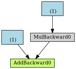
Figure 3: From the graphviz output, we can compile an image of the computational graph
Let’s take a closer look at its components:
- blue boxes
- These correspond to the tensors we use as parameters, the ones we’re asking PyTorch to compute gradients for;
- gray box
- A Python operation that involves a gradient-computing tensor or its dependencies;
- green box
- The same as the gray box, except it is the starting point for
the computation of gradients (assuming the
backward()method is called from the variable used to visualize the graph) — they are computed from the bottom-up in a graph.
Now, take a closer look at the green box: there are two arrows pointing to
it, since it is adding up two variables, a and b*x. Seems obvious, right?
Then, look at the gray box of the same graph: it is performing a
multiplication, namely, b*x. But there is only one arrow pointing to it! The
arrow comes from the blue box that corresponds to our parameter b.
Why don’t we have a box for our data x? The answer is: we do not compute gradients for it! So, even though there are more tensors involved in the operations performed by the computation graph, it only shows gradient-computing tensors and its dependencies.
Try using the make_dot method to plot the computation graph of other
variables, like error or loss.
The only difference between them and the first one is the number of intermediate steps (gray boxes).
dot = make_dot(loss)
dot.format = 'png'
dot.render("/tmp/loss")
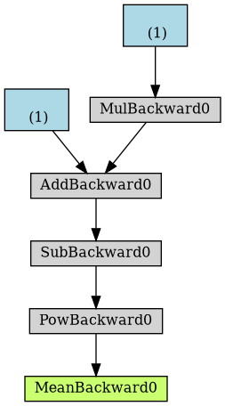
Figure 4: Computational graph from loss
What would happen to the computation graph if we set requires_grad to False
for our parameter a?
a_nograd = torch.randn(1, requires_grad=False, dtype=torch.float, device=device)
b = torch.randn(1, requires_grad=True, dtype=torch.float, device=device)

yhat = a_nograd + b * x_train_tensor
dot = make_dot(yhat)
dot.format = 'png'
dot.render("/tmp/net2")
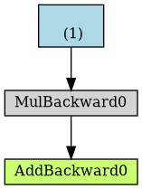
Figure 5: Computational graph from yhat without gradients
Unsurprisingly, the blue box corresponding to the parameter a is no more!
Simple enough: no gradients, no graph.
The best thing about the dynamic computing graph is the fact that you can
make it as complex as you want. You can even use control flow statements
(e.g., if-statements) to control the flow of the gradients (obviously!)
Let’s build a nonsensical, yet complex, computation graph just to make a point!
yhat = a + b * x_train_tensor
error = y_train_tensor - yhat

loss = (error ** 2).mean()

if loss > 0:
    yhat2 = b * x_train_tensor
    error2 = y_train_tensor - yhat2

loss += error2.mean()

dot = make_dot(loss)
dot.format = 'png'
dot.render("/tmp/nonsensical")
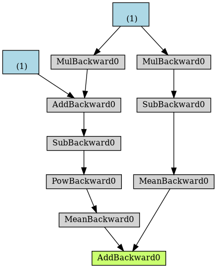
Figure 6: Computational graph of “nonsensical” loss, with if-statement
10. Optimizer: learning the parameters step-by-step pytorch
10.1. Intro
So far, we’ve been manually updating the parameters using the computed gradients. That’s probably fine for two parameters… but what if we had a whole lot of them?! We use one of PyTorch’s optimizers, like SGD or Adam.
There are many optimizers, SGD is the most basic of them and Adam is one of the most popular. They achieve the same goal through, literally, different paths.
Figure 7: Source CS231n Convolutional Neural Networks for Visual Recognition
In the code below, we create a Stochastic Gradient Descent (SGD) optimizer
to update our parameters a and b.
Don’t be fooled by the optimizer’s name: if we use all training data at once for the update — as we are actually doing in the code — the optimizer is performing a batch gradient descent, despite of its name.
# Our parameters
torch.manual_seed(42)
a = torch.randn(1, requires_grad=True, dtype=torch.float, device=device)
b = torch.randn(1, requires_grad=True, dtype=torch.float, device=device)

# Learning rate
lr = 1e-1

# Defines a SGD optimizer to update the parameters
optimizer = optim.SGD([a, b], lr=lr)
10.2. Step / zero_grad
An optimizer takes the parameters we want to update, the learning rate we want to use (and possibly many other hyper-parameters as well) and performs the updates through its step() method.
Besides, we also don’t need to zero the gradients one by one anymore. We just invoke the optimizer’s zero_grad() (so) method and that’s it.
n_epochs = 1000

for epoch in range(n_epochs):
    # Step 1
    yhat = a + b * x_train_tensor

    # Step 2
    error = y_train_tensor - yhat
    loss = (error ** 2).mean()

    # Step 3, compute gradients
    loss.backward()

    # Step 4, apply gradients to update parameters
    # No more manual update!
    # with torch.no_grad():
    #     a -= lr * a.grad
    #     b -= lr * b.grad
    optimizer.step()

    # No more telling PyTorch to let gradients go!
    # a.grad.zero_()
    # b.grad.zero_()
    optimizer.zero_grad()

print(a, b)
Optimization process is now optimized!
Next up is optimizing code for computing the loss.
11. Loss: aggregating erros into a single value pytorch
We now tackle the loss computation. As expected, PyTorch got us covered once again. There are many loss functions to choose from, depending on the task at hand. Since ours is a regression, we are using the Mean Square Error (MSE) loss.
Notice that nn.MSELoss actually creates a loss function for us — it is NOT
the loss function itself. Moreover, you can specify a reduction method to be
applied, that is, how do you want to aggregate the results for individual
points — you can average them (reduction='mean') or simply sum them up
(reduction=’sum’). For example:
# Defines a MSE loss function - function returns a function
loss_fn = nn.MSELoss(reduction='mean')
print(loss_fn)  # --> MSELoss()

fake_labels = torch.tensor([1., 2., 3.])
fake_preds = torch.tensor([1., 3., 5.])
print(loss_fn(fake_labels, fake_preds))  # -->  tensor(1.6667)
We then use the created loss function to compute the loss given our predictions and our labels.
torch.manual_seed(42)
a = torch.randn(1, requires_grad=True, dtype=torch.float, device=device)
b = torch.randn(1, requires_grad=True, dtype=torch.float, device=device)

lr = 1e-1
n_epochs = 1000

# Defines a MSE loss function
loss_fn = nn.MSELoss(reduction='mean')

optimizer = optim.SGD([a, b], lr=lr)

for epoch in range(n_epochs):
    # Step 1
    yhat = a + b * x_train_tensor

    # Step 2
    # No more manual loss!
    # error = y_tensor - yhat
    # loss = (error ** 2).mean()
    loss = loss_fn(y_train_tensor, yhat)

    # Step 3, compute gradients
    loss.backward()

    # Step 4, update parameters using gradients and the learning rate
    optimizer.step()       # update parameters using gradient
    optimizer.zero_grad()  # remove gradient for each parameter

print(a, b)
At this point, there’s only one piece of code left to change: the predictions. It is then time to introduce PyTorch’s way of implementing a…
12. Model: making predictions pytorch
12.1. Introduction
In PyTorch, a model is represented by a regular Python class that inherits from the Module class.
The most fundamental methods it needs to implement are:
- __init__(self)
- Defines the parts that make up the model — in our case,
two parameters,
aandb. - forward(self, x)
- Performs the actual computation, that is, it outputs
a prediction, given the input
x.
Let’s build a proper (yet simple) model for our regression task. It should look like this:
class ManualLinearRegression(nn.Module):
  def __init__(self):
      super().__init__()
      # parameter tensors need their gradient
      a = torch.randn(1, requires_grad=True, dtype=torch.float)
      b = torch.randn(1, requires_grad=True, dtype=torch.float)

      # To make "a" and "b" real parameters of the model, we need to
      # wrap them with nn.Parameter
      self.a = nn.Parameter(a)
      self.b = nn.Parameter(b)

  def forward(self, x):
      # Computes the outputs / predictions
      return self.a + self.b * x
12.2. Parameters
In the _init_ method, we define our two parameters, a and b, using
the Parameter() class, to tell PyTorch these tensors should be considered
parameters of the model they are an attribute of.
Why should we care about that? By doing so, we can use our model’s parameters() method to retrieve an iterator over all model’s parameters, even those parameters of nested models, that we can use to feed our optimizer (instead of building a list of parameters ourselves!).
dummy = ManualLinearRegression()
list(dummy.parameters())
# Returns: [Parameter containing:
# tensor([2.6584], requires_grad=True),
# Parameter containing:
# tensor([1.2004], requires_grad=True)]
Moreover, we can get the current values for all parameters using our
model’s state_dict() method.
dummy.state_dict()
# Returns: OrderedDict([('a', tensor([2.6584])), ('b', tensor([1.2004]))])
nil
12.3. state_dict
The state_dict() of a given model is simply a Python dictionary that maps
each layer / parameter to its corresponding tensor. But only learnable
parameters are included, as its purpose is to keep track of parameters that
are going to be updated by the optimizer.
The optimizer itself also has a state_dict(), which contains its
internal state, as well as the hyperparameters used.
It turns out state_dicts can also be used for checkpointing a model, as we will see later down the line.
optimizer.state_dict()
Returns:
{'state': {},
 'param_groups': [{'lr': 0.1,
   'momentum': 0,
   'dampening': 0,
   'weight_decay': 0,
   'nesterov': False,
   'params': [0, 1]}]}
12.4. Device
IMPORTANT: we need to send our model to the same device where the data is. If our data is made of GPU tensors, our model must “live” inside the GPU as well.
torch.manual_seed(42)
device = 'cuda' if torch.cuda.is_available() else 'cpu'

# Now we can create a model and send it at once to the device
model = ManualLinearRegression().to(device)

# We can also inspect its parameters using its state_dict
print(model.state_dict())
12.5. Forward Pass
The forward pass is the moment when the model makes predictions.
You should NOT call the forward(x) method, though. You should call the
whole model itself, as in model(x) to perform a forward pass and output
predictions.
yhat = model(x_train_tensor)
12.6. Train
In PyTorch, models have a train() method which, somewhat disappointingly,
does NOT perform a training step. Its only purpose is to set the model to
training mode (so).
Why is this important? Some models may use mechanisms like Dropout, for instance, which have distinct behaviors in training and evaluation phases.
lr = 1e-1
n_epochs = 1000

loss_fn = nn.MSELoss(reduction='mean')

# Now the optimizers uses the parameters from the model
optimizer = optim.SGD(model.parameters(), lr=lr)

for epoch in range(n_epochs):
    # Sets model to training mode
    model.train()

    # Step 1
    # No more manual prediction!
    # yhat = a + b * x_tensor
    yhat = model(x_train_tensor)

    # Step 2, compute loss, sum of errors
    loss = loss_fn(yhat, y_train_tensor)
    # Step 3, compute gradients
    loss.backward()
    # Step 4, update parameters, and zero out gradient
    optimizer.step()
    optimizer.zero_grad()

print(model.state_dict())
Now, the printed statements will look like this
OrderedDict([('0.weight', tensor([[1.9690]], device='cuda:0')),
             ('0.bias', tensor([1.0235], device='cuda:0'))])
final values for parameters a and b are still the same, so everything
is OK.
12.7. Nested Models
In our model, we manually created two parameters to perform a linear regression.
You are not limited to defining parameters, though: models can contain other models as its attributes as well, so you can easily nest them. We’ll see an example of this shortly as well.
Let’s use PyTorch’s Linear model as an attribute of our own, thus creating a nested model.
Even though this clearly is a contrived example, as we are pretty much wrapping the underlying model without adding anything useful (or, at all!) to it, it illustrates the concept well.
In the __init__ method, we created an attribute that contains our nested
Linear model.
In the forward() method, we call the nested model itself to perform the
forward pass (notice, we are not calling self.linear.forward(x)!).
class LayerLinearRegression(nn.Module):
    def __init__(self):
        super().__init__()
        # Instead of our custom parameters, we use a Linear layer with
        # single input and single output
        self.linear = nn.Linear(1, 1)

    def forward(self, x):
        # Now it only takes a call to the layer to make predictions
        return self.linear(x)
Now, if we call the parameters() method of this model, PyTorch will
figure the parameters of its attributes in a recursive way.
You can also add new Linear attributes and, even if you don’t use them at
all in the forward pass, they will still be listed under parameters().
dummy = LayerLinearRegression()
list(dummy.parameters())
# -> OrderedDict([('linear.weight', tensor([[0.4591]])),
#                 ('linear.bias', tensor([-0.7359]))])
dummy.state_dict()
# -> LayerLinearRegression( (linear): Linear(in_features=1, out_features=1, bias=True))
12.8. Layers
A Linear model can be seen as a layer in a neural network.
3 -> 4 -> 1 ->
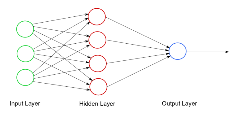
Figure 8: Neural network
In the example above, the hidden layer would be nn.Linear(3, 4) and the
output layer would be nn.Linear(4, 1).
There are MANY different layers that can be uses in PyTorch:
- Convolution Layers
- Pooling Layers
- Padding Layers
- Non-linear Activations
- Normalization Layers
- Recurrent Layers
- Transformer Layers
- Linear Layers
- Dropout Layers
- Sparse Layers (embbedings)
- Vision Layers
- DataParallel Layers (multi-GPU)
- Flatten Layer
We have just used a Linear layer.
12.9. Sequential Models
Our model was simple enough… You may be thinking: “why even bother to build a class for it?!” Well, you have a point…
For straightforward models, that use run-of-the-mill layers, where the output of a layer is sequentially fed as an input to the next, we can use a Sequential model
In our case, we would build a Sequential model with a single argument, that is, the Linear layer we used to train our linear regression. The model would look like this:
model = nn.Sequential(nn.Linear(1, 1)).to(device)
Simple enough, right?
12.10. Defining Training step-function
So far, we’ve defined:
- An optimizer
- A loss function
- A model
Scroll up a bit and take a quick look at the code inside the loop. Would it change if we were using a different optimizer, or loss, or even model? If not, how can we make it more generic?
Well, I guess we could say all these lines of code perform a training step, given those three elements (optimizer, loss and model), the features and the labels.
So, how about writing a function that takes those three elements and returns another function that performs a training step, taking a set of features and labels as arguments and returning the corresponding loss?
def make_train_step(model, loss_fn, optimizer):
    # Builds function that performs a step in the train loop
    def train_step(x, y):
        # Sets model to TRAIN mode
        model.train()
        # Step 1: Make predictions
        yhat = model(x)
        # Step 2: Compute loss
        loss = loss_fn(yhat, y)
        # Step 3: Compute gradients
        loss.backward()
        # Step 4: Update parameters and zeroes gradients
        optimizer.step()
        optimizer.zero_grad()
        # Returns the loss
        return loss.item()

    # Returns the function that will be called inside the train loop
    return train_step
Then we can use this general-purpose function to build a train_step()
function to be called inside our training loop.
lr = 1e-1

# Create a MODEL, a LOSS FUNCTION and an OPTIMIZER
model = nn.Sequential(nn.Linear(1, 1)).to(device)
loss_fn = nn.MSELoss(reduction='mean')
optimizer = optim.SGD(model.parameters(), lr=lr)

# Create the train_step function for our model, loss function and optimizer
train_step = make_train_step(model, loss_fn, optimizer)
The training loop now becomes significantly cleaner
n_epochs = 1000

losses = []
# For each epoch...
for epoch in range(n_epochs):
    # Performs one train step and returns the corresponding loss
    loss = train_step(x_train_tensor, y_train_tensor)
    losses.append(loss)

# Checks model's parameters
print(model.state_dict())

plt.plot(losses[:200])
plt.xlabel('Epochs')
plt.ylabel('Loss')
plt.yscale('log')
plt.savefig('/tmp/trainingloss.png', bbox_inches="tight")
Let’s give our training loop a rest and focus on our data for a while: So far, we’ve simply used our Numpy arrays turned PyTorch tensors. But we can do better, we can build a…
13. Dataset dataset
In PyTorch, a dataset is represented by a regular Python class that inherits from the Dataset class. You can think of it as a kind of a Python list of tuples, each tuple corresponding to one point (features, label).
The most fundamental methods it needs to implement are:
__init__(self): It takes whatever arguments needed to build a list of tuples — it may be the name of a CSV file that will be loaded and processed; it may be two tensors, one for features, another one for labels; or anything else, depending on the task at hand.__get_item__(self, index): It allows the dataset to be indexed, so it can work like a list (dataset[i]) — it must return a tuple (features, label) corresponding to the requested data point. We can either return the corresponding slices of our pre-loaded dataset or tensors or, as mentioned above, load them on demand (like in this example).__len__(self): It should simply return the size of the whole dataset so, whenever it is sampled, its indexing is limited to the actual size.
There is no need to load the whole dataset in the constructor method
(__init__). If your dataset is big (tens of thousands of image files, for
instance), loading it at once would not be memory efficient. It is
recommended to load them on demand (whenever __get_item__ is called).
Let’s build a simple custom dataset that takes two tensors as arguments: one for the features, one for the labels. For any given index, our dataset class will return the corresponding slice of each of those tensors. It should look like this:
from torch.utils.data import Dataset

class CustomDataset(Dataset):
  def __init__(self, x_tensor, y_tensor):
      self.x = x_tensor
      self.y = y_tensor

  def __getitem__(self, index):
      return (self.x[index], self.y[index])

  def __len__(self):
      return len(self.x)

# Wait, is this a CPU tensor now? Why? Where is .to(device)?
x_train_tensor = torch.from_numpy(x_train).float()
y_train_tensor = torch.from_numpy(y_train).float()

train_data = CustomDataset(x_train_tensor, y_train_tensor)
print(train_data[0])  # --> (tensor([0.7713]), tensor([2.4745]))
Did you notice we built our training tensors out of Numpy arrays but we did not send them to a device? So, they are CPU tensors now! Why?
We don’t want our whole training data to be loaded into GPU tensors, as we have been doing in our example so far, because it takes up space in our precious graphics card’s RAM.
13.1. TensorDataset
Besides, you may be thinking “why go through all this trouble to wrap a couple of tensors in a class?”. And, once again, you do have a point… if a dataset is nothing else but a couple of tensors, we can use PyTorch’s TensorDataset class, which will do pretty much what we did in our custom dataset above.
from torch.utils.data import TensorDataset
train_data = TensorDataset(x_train_tensor, y_train_tensor)
print(train_data[0])
OK, fine, but then again, why are we building a dataset anyway? We’re doing it because we want to use a…
14. DataLoader, splitting your data into mini-batches
- Let’s split data into mini-batches
- Use DataLoaders!
Until now, we have used the whole training data at every training step. It has been batch gradient descent all along. This is fine for our ridiculously small dataset, sure, but if we want to get serious about all this, we must use mini-batch gradient descent. Thus, we need mini-batches. Thus, we need to slice our dataset accordingly.
Do you want to do it manually?! Me neither!
So we use PyTorch’s DataLoader class for this job. We tell it which dataset to use (the one we just built in the previous section), the desired mini-batch size and if we’d like to shuffle it or not. That’s it!
Our loader will behave like an iterator, so we can loop over it and fetch a different mini-batch every time.
from torch.utils.data import DataLoader
train_loader = DataLoader(dataset=train_data, batch_size=16, shuffle=True)
To retrieve a sample mini-batch, one can simply run the command below — it will return a list containing two tensors, one for the features, another one for the labels.
next(iter(train_loader))
How does this change our training loop? Let’s check it out!
lr = 1e-1

# Create a MODEL, a LOSS FUNCTION and an OPTIMIZER
model = nn.Sequential(nn.Linear(1, 1)).to(device)
loss_fn = nn.MSELoss(reduction='mean')
optimizer = optim.SGD(model.parameters(), lr=lr)

# Create the train_step function for our model, loss function and optimizer
train_step = make_train_step(model, loss_fn, optimizer)

n_epochs = 1000

losses = []

for epoch in range(n_epochs):
    # inner loop
    for x_batch, y_batch in train_loader:
        # the dataset "lives" in the CPU, so to do our mini-batches,
        # we need to send those mini-batches to the device where the
        # model "lives"
        x_batch = x_batch.to(device)
        y_batch = y_batch.to(device)

        loss = train_step(x_batch, y_batch)
        losses.append(loss)

print(model.state_dict())

plt.plot(losses)
plt.xlabel('Epochs (?)')
plt.ylabel('Loss')
plt.yscale('log')
plt.show()
Did you notice it is taking longer to train now? Can you guess why?
Two things are different now: not only do we have an inner loop to load each and every mini-batch from our DataLoader but, more importantly, we are now sending only one mini-batch to the device.
For bigger datasets, loading data sample by sample (into a CPU tensor) using
Dataset’s _get_item_ and then sending all samples that belong to the same
mini-batch at once to your GPU (device) is the way to go in order to make
the best use of your graphics card’s RAM.
Moreover, if you have many GPUs to train your model on, it is best to keep your dataset “agnostic” and assign the batches to different GPUs during training.
So far, we’ve focused on the training data only. We built a dataset and a
data loader for it. We could do the same for the validation data, using the
split we performed at the beginning of this post… or we could use
random_split instead.
14.1. random_split
PyTorch’s random_split() method is an easy and familiar way of performing
a training-validation split. Just keep in mind that, in our example, we
need to apply it to the whole dataset (not the training dataset we built
a few sections ago).
Then, for each subset of data, we build a corresponding DataLoader, so our code looks like this:
from torch.utils.data.dataset import random_split

# build tensors from numpy arrays BEFORE split
x_tensor = torch.from_numpy(x).float()
y_tensor = torch.from_numpy(y).float()

# build dataset containing ALL data points
dataset = TensorDataset(x_tensor, y_tensor)

# perform the split (could do, e.g. a [60,20,20] split as well)
train_dataset, val_dataset = random_split(dataset, [80, 20])

# build a loader of each set
train_loader = DataLoader(dataset=train_dataset, batch_size=16)
val_loader = DataLoader(dataset=val_dataset, batch_size=20)
Now we have a data loader for our validation set, so, it makes sense to use it for the…
14.2. Big WARNING
When combining pytorch and numpy code, there is a bug that is very common (of a 1000 analyzed github repositories, 95% suffered, even pytorch’s own tutorial!), explained here: Using PyTorch + NumPy? You’re making a mistake
15. Evaluation: does it generalize?
Now, we need to change the training loop to include the evaluation of our model, that is, computing the validation loss. The first step is to include another inner loop to handle the mini-batches that come from the validation loader, sending them to the same device as our model. Next, we make predictions using our model and compute the corresponding loss.
That’s pretty much it, but there are two small, yet important, things to consider:
- torch.no_grad(): even though it won’t make a difference in our simple model, it is a good practice to wrap the validation inner loop with this context manager to disable any gradient calculation that you may inadvertently trigger - gradients belong in training, not in validation steps;
- eval(): the only thing it does is setting the model to evaluation mode
(just like its
train()counterpart did), so the model can adjust its behavior regarding some operations, like Dropout.
Now, our training loop should look like this:
torch.manual_seed(42)

# build tensors from numpy arrays BEFORE split
x_tensor = torch.from_numpy(x).float()
y_tensor = torch.from_numpy(y).float()

# build dataset containing ALL data points
dataset = TensorDataset(x_tensor, y_tensor)

# perform the split
train_dataset, val_dataset = random_split(dataset, [80, 20])

# build a loader of each set
train_loader = DataLoader(dataset=train_dataset, batch_size=16)
val_loader = DataLoader(dataset=val_dataset, batch_size=20)

# define learning rate
lr = 1e-1

# Create a MODEL, a LOSS FUNCTION and an OPTIMIZER
model = nn.Sequential(nn.Linear(1, 1)).to(device)
loss_fn = nn.MSELoss(reduction='mean')
optimizer = optim.SGD(model.parameters(), lr=lr)

# Create the train_step function for our model, loss function and optimizer
train_step = make_train_step(model, loss_fn, optimizer)

n_epochs = 1000

losses = []
val_losses = []

# Looping through epochs...
for epoch in range(n_epochs):
    # TRAINING
    batch_losses = []
    for x_batch, y_batch in train_loader:
        x_batch = x_batch.to(device)
        y_batch = y_batch.to(device)

        loss = train_step(x_batch, y_batch)
        batch_losses.append(loss)

    losses.append(np.mean(batch_losses))

    # VALIDATION
    # no gradients in validation!
    with torch.no_grad():
        val_batch_losses = []
        for x_val, y_val in val_loader:
            x_val = x_val.to(device)
            y_val = y_val.to(device)

            # sets model to EVAL mode
            model.eval()

            # make predictions
            yhat = model(x_val)
            val_loss = loss_fn(yhat, y_val)
            val_batch_losses.append(val_loss.item())

        val_losses.append(np.mean(val_batch_losses))

print(model.state_dict())
plt.figure()
plt.xlim(0, 100)
plt.xlabel('Epochs')
plt.ylabel('Loss')
plt.yscale('log')
plt.plot(losses, label='Training Loss', linestyle="-", linewidth=2)
plt.plot(val_losses, label='Validation Loss', linestyle=":", linewidth=2)
plt.legend()
plt.savefig("/tmp/train_val_curves2.png", bbox_inches="tight")
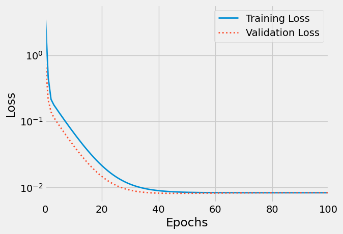
Figure 9: Train/validation curves
“Wait, there is something weird with this plot…”, you say. You’re right, the validation loss is smaller than the training loss. Shouldn’t it be the other way around?! Well, generally speaking, YES, it should… but you can learn more about situations where this swap happens at this great post.
16. Training Loop
The training loop should be a stable structure, so we can organize it into functions as well… Let’s build a function for validation and another one for the training loop itself, training step and all!
def make_train_step(model, loss_fn, optimizer):
    # Builds function that performs a step in the train loop
    def train_step(x, y):
        # Sets model to TRAIN mode
        model.train()
        # Step 1: Makes predictions
        yhat = model(x)
        # Step 2: Compute loss
        loss = loss_fn(yhat, y)
        # Step 3: Compute gradients
        loss.backward()
        # Step 4: Update parameters and zeroes gradients
        optimizer.step()
        optimizer.zero_grad()
        # Return the loss
        return loss.item()

    # Returns the function that will be called inside the train loop
    return train_step


def validation(model, loss_fn, val_loader):
    # Figures device from where the model parameters (hence, the model) are
    device = next(model.parameters()).device.type

    # no gradients in validation!
    with torch.no_grad():
        val_batch_losses = []
        for x_val, y_val in val_loader:
            x_val = x_val.to(device)
            y_val = y_val.to(device)

            # set model to EVAL mode
            model.eval()

            # make predictions
            yhat = model(x_val)
            val_loss = loss_fn(yhat, y_val)
            val_batch_losses.append(val_loss.item())

        val_losses = np.mean(val_batch_losses)

    return val_losses


def train_loop(model, loss_fn, optimizer, n_epochs, train_loader, val_loader=None):
    # Device from where the model parameters (hence, the model) are
    device = next(model.parameters()).device.type
    # Create the train_step function for our model, loss function and optimizer
    train_step = make_train_step(model, loss_fn, optimizer)

    losses = []
    val_losses = []

    for epoch in range(n_epochs):
        # TRAINING
        batch_losses = []
        for x_batch, y_batch in train_loader:
            x_batch = x_batch.to(device)
            y_batch = y_batch.to(device)

            loss = train_step(x_batch, y_batch)
            batch_losses.append(loss)

        losses.append(np.mean(batch_losses))

        # VALIDATION
        if val_loader is not None:
            val_loss = validation(model, loss_fn, val_loader)
            val_losses.append(val_loss)

        print("Epoch {} complete...".format(epoch))

    return losses, val_losses
17. Final Code
We finally have an organized version of our code, consisting of the following steps:
- building a Dataset
- performing a random split into train and validation datasets
- building DataLoaders
- building a model
- defining a loss function
- specifying a learning rate
- defining an optimizer
- specifying the number of epochs
All nitty-gritty details of performing the actual training is encapsulated
inside the train_loop function.
device = 'cuda' if torch.cuda.is_available() else 'cpu'
torch.manual_seed(42)

# builds tensors from numpy arrays BEFORE split
x_tensor = torch.from_numpy(x).float()
y_tensor = torch.from_numpy(y).float()

# builds dataset containing ALL data points
dataset = TensorDataset(x_tensor, y_tensor)

# performs the split
train_dataset, val_dataset = random_split(dataset, [80, 20])

# builds a loader of each set
train_loader = DataLoader(dataset=train_dataset, batch_size=16)
val_loader = DataLoader(dataset=val_dataset, batch_size=20)

# defines learning rate
lr = 1e-1

# Create a MODEL, a LOSS FUNCTION and an OPTIMIZER
model = nn.Sequential(nn.Linear(1, 1)).to(device)
loss_fn = nn.MSELoss(reduction='mean')
optimizer = optim.SGD(model.parameters(), lr=lr)

n_epochs = 1000

losses, val_losses = train_loop(model, loss_fn, optimizer, n_epochs, train_loader, val_loader)

print(model.state_dict())
plt.plot(losses, label='Training Loss', linestyle="-", linewidth=2)
plt.plot(val_losses, label='Validation Loss', linestyle=":", linewidth=2)
plt.yscale('log')
plt.xlabel('Epochs')
plt.ylabel('Loss')
plt.legend()
plt.savefig("/tmp/train_val_curves.png", bbox_inches="tight")
plt.show()
18. BONUS: Further Improvements
Is there anything else we can improve or change? Sure, there is always something else to add to your model, like save/load or using a learning rate scheduler, for instance.
18.1. Saving (and Loading) Models: taking a break
So, it is important to be able to checkpoint our model, in case we’d like to restart training later.
To checkpoint a model, we basically have to save its state into a file, to load it back later - nothing special, actually.
What defines the state of a model?
model.state_dict(): kinda obvious, right?optimizer.state_dict(): remember optimizers had the state_dict as well?loss: after all, you should keep track of its evolutionepoch: it is just a number, so why not? :-)- anything else you’d like to have restored
Then, wrap everything into a Python dictionary and use torch.save() to dump it all into a file!
checkpoint = {'epoch': n_epochs,
              'model_state_dict': model.state_dict(),
              'optimizer_state_dict': optimizer.state_dict(),
              'loss': losses,
              'val_loss': val_losses}

torch.save(checkpoint, 'model_checkpoint.pth')
How would you load it back? Easy as well:
- load the dictionary back using torch.load()
- load model and optimizer state dictionaries back using its methods load_state_dict()
- load everything else into their corresponding variables
checkpoint = torch.load('model_checkpoint.pth')

model.load_state_dict(checkpoint['model_state_dict'])
optimizer.load_state_dict(checkpoint['optimizer_state_dict'])

epoch = checkpoint['epoch']
losses = checkpoint['loss']
val_losses = checkpoint['val_loss']
You may save a model for checkpointing, like we have just done, or for making predictions, assuming training is finished.
After loading the model, DO NOT FORGET:
SET THE MODE:
checkpointing: model.train()
predicting: model.eval()
18.2. Learning Rate Scheduler
NOTE: the cool kids use Adabound optimizers (and no scheduler) these days.
In the “Playing with the Learning Rate” section, we observed how different learning rates may be more useful at different moments of the optimization process.
PyTorch offers a long list of learning rate schedulers for all your learning rate needs:
- StepLR
- MultiStepLR
- ReduceLROnPlateau
- LambdaLR
- ExponentialLR
- CosineAnnealingLR
- CyclicLR
- OneCycleLR
- CosineAnnealingWarmRestarts (this seems to be one of the best)
To include a scheduler into our workflow, we need to take two steps:
- create a scheduler and pass our optimizer as argument
- use our scheduler’s
step()method- after the validation, that is, last thing before finishing an epoch, for the first 6 schedulers on the list
- after every batch update for the last 3 schedulers on the list
We also need to pass an argument to step() if we’re using
ReduceLROnPlateau: the validation loss, which is the quantity we’re using
to control the effectiveness of the current learning rate.
from torch.optim.lr_scheduler import StepLR, ReduceLROnPlateau, MultiStepLR

optimizer = optim.SGD(model.parameters(), lr=lr)
scheduler = ReduceLROnPlateau(optimizer, 'min')

#scheduler = StepLR(optimizer, step_size=30, gamma=0.5)
#scheduler = MultiStepLR(optimizer, milestones=[30,80], gamma=0.1)
We are focusing only on ReduceLROnPlateau, StepLR and MultiStepLR on
this tutorial, so we’ll change our training loop accordingly: adding the
scheduler’s step() as last thing before finishing an epoch.
def train_loop_with_scheduler(model, loss_fn, optimizer, scheduler, n_epochs, train_loader, val_loader=None):
    # Device from where the model parameters (hence, the model) are
    device = next(model.parameters()).device.type
    # Create the train_step function for our model, loss function and optimizer
    train_step = make_train_step(model, loss_fn, optimizer)

    losses = []
    val_losses = []
    learning_rates = []

    for epoch in range(n_epochs):
        # TRAINING
        batch_losses = []
        for x_batch, y_batch in train_loader:
            x_batch = x_batch.to(device)
            y_batch = y_batch.to(device)

            loss = train_step(x_batch, y_batch)
            batch_losses.append(loss)

        losses.append(np.mean(batch_losses))

        # VALIDATION
        if val_loader is not None:
            val_loss = validation(model, loss_fn, val_loader)
            val_losses.append(val_loss)

        print(f"Epoch {epoch} complete...")

        # SCHEDULER
        if isinstance(scheduler, torch.optim.lr_scheduler.ReduceLROnPlateau):
            scheduler.step(val_loss)
        else:
            scheduler.step()

        learning_rates.append(optimizer.state_dict()['param_groups'][0]['lr'])

    return losses, val_losses, learning_rates
Let’s run the whole thing once again!
torch.manual_seed(42)

# builds tensors from numpy arrays BEFORE split
x_tensor = torch.from_numpy(x).float()
y_tensor = torch.from_numpy(y).float()

# builds dataset containing ALL data points
dataset = TensorDataset(x_tensor, y_tensor)

# performs the split
train_dataset, val_dataset = random_split(dataset, [80, 20])

# builds a loader of each set
train_loader = DataLoader(dataset=train_dataset, batch_size=16)
val_loader = DataLoader(dataset=val_dataset, batch_size=20)

# defines learning rate
lr = 1e-1

# Create a MODEL, a LOSS FUNCTION and an OPTIMIZER (and SCHEDULER)
model = nn.Sequential(nn.Linear(1, 1)).to(device)
loss_fn = nn.MSELoss(reduction='mean')
optimizer = optim.SGD(model.parameters(), lr=lr)

scheduler = ReduceLROnPlateau(optimizer, 'min')
#scheduler = StepLR(optimizer, step_size=30, gamma=0.5)
#scheduler = MultiStepLR(optimizer, milestones=[30,80], gamma=0.1)

n_epochs = 1000

losses, val_losses, l_rates = train_loop_with_scheduler(model, loss_fn, optimizer, scheduler, n_epochs, train_loader, val_loader)

print(model.state_dict())
18.3. plots
As expected, the learning rate is progressively reduced.
fig, ax1 = plt.subplots()
ax2_col = "green"
ax1.set_xlim(0, 100)
ax2 = ax1.twinx()

ax1.plot(losses, label='Training Loss', linestyle="-", linewidth=2)
ax1.plot(val_losses, label='Validation Loss', linestyle=":", linewidth=2)
ax1.set_xlabel('Epochs')
ax1.set_ylabel('Loss')
ax1.set_yscale("log")

ax2.set_yscale("log")
ax2.plot(l_rates, label='Learning rate', linestyle="--", linewidth=1, color=ax2_col)
ax2.set_ylabel('Learning Rate', color=ax2_col)
ax2.tick_params(axis='y', labelcolor=ax2_col)

ax1.legend()
fig.tight_layout()
fig.savefig("/tmp/lr_scheduler.png", bbox_inches="tight")
plt.show()
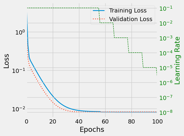
Figure 10: Learning rate (green) is reduced with increasing epochs
18.4. Multiple parallelism
It’s natural to execute your forward, backward propagations on multiple GPUs. However, Pytorch will only use one GPU by default. You can easily run your operations on multiple GPUs by making your model run in parallel using DataParallel:
model = nn.DataParallel(model)
18.4.1. Dummy dataset
Small example:
import torch
import torch.nn as nn
from torch.utils.data import Dataset, DataLoader

# Parameters and DataLoaders
input_size = 5
output_size = 2

batch_size = 30
data_size = 100

device = torch.device("cuda:0" if torch.cuda.is_available() else "cpu")

# Make dummy dataset, just needs a __getitem__ method:
class RandomDataset(Dataset):

    def __init__(self, size, length):
        self.len = length
        self.data = torch.randn(length, size)

    def __getitem__(self, index):
        return self.data[index]

    def __len__(self):
        return self.len

rand_loader = DataLoader(dataset=RandomDataset(input_size, data_size),
                         batch_size=batch_size, shuffle=True)
18.4.2. Simple Model
For the demo, our model just gets an input, performs a linear operation,
and gives an output. However, you can use DataParallel on any model (CNN,
RNN, Capsule Net etc.)
We’ve placed a print statement inside the model to monitor the size of input and output tensors. Please pay attention to what is printed at batch rank 0.
class Model(nn.Module):
    # Our model

    def __init__(self, input_size, output_size):
        super(Model, self).__init__()
        self.fc = nn.Linear(input_size, output_size)

    def forward(self, input):
        output = self.fc(input)
        print("\tIn Model: input size", input.size(),
              "output size", output.size())

        return output
18.4.3. Create Model and DataParallel
This is the core part of the tutorial. First, we need to make a model
instance and check if we have multiple GPUs. If we have multiple GPUs, we
can wrap our model using nn.DataParallel. Then we can put our model on
GPUs by model.to(device).
model = Model(input_size, output_size)
if torch.cuda.device_count() > 1:
    print(f"Let's use {torch.cuda.device_count()} GPUs!")
    # dim = 0 [30, xxx] -> [10, ...], [10, ...], [10, ...] on 3 GPUs
    model = nn.DataParallel(model)

model.to(device)

for data in rand_loader:
    input = data.to(device)
    output = model(input)
    print(f"Outside: input size {input.size()} output_size {output.size()}")
18.5. Hyperparameter search
Using PyTorch’s Ax, as described in tutorial
pip3 install ax-platform
or bleeding edge:
pip3 install 'git+https://github.com/facebook/Ax.git#egg=Ax'
from ax import optimize
best_parameters, best_values, _, _ = optimize(
    parameters=[
        {"name": "x1",
         "type": "range",
         "bounds": [-10.0, 10.0],},
        {"name": "x2",
         "type": "range",
         "bounds": [-10.0, 10.0],},],
    evaluation_function=booth,
    minimize=True,)print(best_parameters)
19. Appendix 0: Some overview
Some useful resources:
| Package | Description |
|---|---|
| torch | The top-level PyTorch package and tensor library. |
| torch. nn | A subpackage that contains modules and extensible classes for |
| building neural networks. | |
| torch.autograd | A subpackage that supports all the differentiable Tensor operations in |
| PyTorch.torch.nn.functional | A functional interface that contains typical operations used for |
| building neural networks like loss functions, activation functions, | |
| and convolution operations. | |
| torch.optim | A subpackage that contains standard optimization operations like SGD and Adam. |
| torch.utils | A subpackage that contains utility classes like data sets and |
| data loaders that make data preprocessing easier. | |
| torchvision | A package that provides access to popular datasets, |
| model architectures, and image transformations for computer vision. |
| Data type | dtype | CPU tensor | GPU tensor |
|---|---|---|---|
| 32-bit floating point | torch.float32 or torch.float | torch.FloatTensor | torch.cuda.FloatTensor |
| 64-bit floating point | torch.float64 or torch.double | torch.DoubleTensor | torch.cuda.DoubleTensor |
| 16-bit floating point | torch.float16 or torch.half | torch.HalfTensor | torch.cuda.HalfTensor |
| 8-bit integer (unsigned) | torch.uint8 | torch.ByteTensor | torch.cuda.ByteTensor |
| 8-bit integer (signed) | torch.int8 | torch.CharTensor | torch.cuda.CharTensor |
| 16-bit integer (signed) | torch.int16 or torch.short | torch.ShortTensor | torch.cuda.ShortTensor |
| 32-bit integer (signed) | torch.int32 or torch.int | torch.IntTensor | torch.cuda.IntTensor |
| 64-bit integer (signed) | torch.int64 or torch.long | torch.LongTensor | torch.cuda.LongTensor |
| Boolean | torch.bool | torch.BoolTensor | torch.cuda.BoolTensor |
20. Appendix A: Further
These are my own notes, for further reading, see https://pytorch.org/tutorials/
Tutorial to read:
- Why PyTorch? tutorial
- Autograd: automatic differentiation tutorial
- Neural Networks tutorial
- Training a classifier tutorial
- Optional: Data Parallelism tutorial
- Annotated PyTorch guide (Looks excellent for beginners)
Things I need to look into:
- Autoencoder in pytorch
- TensorBoard (tutorial)
- Hyperopt
- Multiple outputs from an ANN?
- TorchScript (tutorial)
- For converting Pytorch models for high performance deployment, allows for compiler optimizations, no Global Interpreter Lock
- TorchVision - for image recognition
torchvision.datasetshas loaders for Imagenet, CIFAR10, MNIST… impaired
21. Appendix B: Autoencoder
- One of the best ML write-ups on Autoencoders is the one on keras’ blog.
- For variational auto-encoder, see https://graviraja.github.io/vanillavae/
- Other VAE: https://github.com/L1aoXingyu/pytorch-beginner/tree/master/08-AutoEncoder
Misc:
nn.ReLU()vsnn.functional.relu()see: https://discuss.pytorch.org/t/whats-the-difference-between-nn-relu-vs-f-relu/27599
Here, we’ll build an Autoencoder for the MNIST dataset.
21.1. TODO Left to play with
- Get parameters of embedding layer?
- use actual labels in embedding_plot
- use all data for embedding plot, not just single batch.
- Add learning rate scheduler?
- Add sparcity constraint, in keras: “activity_regularizer”
- Hyperopt?
- make_dot
- visualize graph betterh than make_dot
- Separate encoder from decoder
- Play with conv net instead?
21.2. Head
Import libraries and parameters. Code based on example from Dimension Manipulation using Autoencoder in Pytorch on MNIST dataset
import numpy as np
import torch
import torch.optim as optim
import torch.nn as nn
import torchvision as tv

import torch.nn.functional as F
from torch.utils.data import DataLoader

from torchviz import make_dot
from torch.optim.lr_scheduler import ReduceLROnPlateau

epochs = 20
batch_size = 32
path = "/tmp"

# Compression of factor 24.5, assuming the input is 784 float
embedding_dim = 32
21.3. Define Neural Network — version 1
Here we use the Linear() module form PyTorch, to model a fully connected layer, here in matrix representation:
\begin{equation*} \boldsymbol{y} = \boldsymbol{xA}^{T} + b \end{equation*}
Modules that have a state (parameters) are defined in __init__ such that
parameters are owned by the model, and can be trained. For the forward()
method, we may use the methods in the functional library
torch.nn.functional, but it really doesn’t matter, for instance
nn.ReLU() and F.relu() are the same, but the former creates a module
that can be added to nn.Sequential() as we’ll see in next section, while
the latter is just a x=max(0,x)
class autoencoder(nn.Module):
    def __init__(self, dim=32, **kwargs):
        super().__init__()
        assert(dim <= 64)

        # Note: We define the nn.<model> in __init__ because they have
        # learnable parameters. Most handy to use the torch.nn module
        # for that.

        # Encoder, 4 fully connected / "dense" layers
        self.fc1 = nn.Linear(kwargs["input_shape"], 128)
        self.fc2 = nn.Linear(128, 64)
        self.fc3 = nn.Linear(64, dim)

        # Decoder, the encoder in reverse
        self.fc6 = nn.Linear(dim, 64)
        self.fc7 = nn.Linear(64, 128)
        self.fc8 = nn.Linear(128, kwargs["input_shape"])

    def forward(self, x):
        # Pooling and ReLU don't have learnable parameters, so usually
        # goes here. More convinient to use torch.nn.functional for them.

        # Encoder
        x = self.fc1(x)
        x = F.relu(x)         # (ReLU(x) = max(0,x))

        x = self.fc2(x)
        x = F.relu(x)

        x = self.fc3(x)
        x = F.relu(x)

        # Decoder
        x = self.fc6(x)
        x = F.relu(x)

        x = self.fc7(x)
        x = F.relu(x)

        x = self.fc8(x)
        # Output layer, for scaling between 0 to 1
        # x = torch.sigmoid(x)
        x = torch.tanh(x)
        return x
Access hidden layer by, e.g.:
model = autoencoder(32, input_shape=28*28)
model.fc3.weight
21.4. Define Neural Network — version 2, , using ’Sequential’
Here we use nn.Sequential() to pass the output of one module as input to
the next, giving a more compact and easier notation. (There’s also
nn.ModuleList() with similar use-case.)
class autoencoder(nn.Module):
    def __init__(self, dim=32, **kwargs):
        super().__init__()
        self.encoder = nn.Sequential(
            nn.Linear(kwargs["input_shape"], 128),
            nn.ReLU(True),
            nn.Linear(128, 64),
            nn.ReLU(True),
            nn.Linear(64, dim))
        self.decoder = nn.Sequential(
            nn.Linear(dim, 64),
            nn.ReLU(True),
            nn.Linear(64, 128),
            nn.ReLU(True),
            nn.Linear(128, kwargs["input_shape"]),
            nn.Tanh())

    def forward(self, x):
        x = self.encoder(x)
        x = self.decoder(x)
        return x
Access hidden layer by:
model = autoencoder(32, input_shape=28*28)
model.encoder[4].weight
print(model.encoder)
 Sequential(
   (0): Linear(in_features=784, out_features=128, bias=True)
   (1): ReLU(inplace=True)
   (2): Linear(in_features=128, out_features=64, bias=True)
   (3): ReLU(inplace=True)
   (4): Linear(in_features=64, out_features=32, bias=True))
21.5. Initiate model, and helper functions
Initiate model, optimizer and loss-function
def to_img(x):
    "De-Normalize MNIST images, for checking training"
    x = 0.5 * (x + 1)
    x = x.clamp(0, 1)
    x = x.view(x.size(0), 1, 28, 28)
    return x

# use GPU if available
device = torch.device("cuda" if torch.cuda.is_available() else "cpu")

# create a model from `AE` autoencoder class
# load it to the specified device, either gpu or cpu
# model = ae(embedding_dim, input_shape=28*28).to(device)
model = autoencoder(embedding_dim, input_shape=28*28).to(device)

# create an optimizer object
# Adam optimizer with learning rate 1e-3; can also play with weight_decay=1e-5
optimizer = optim.Adam(model.parameters(), lr=1e-3)

# Mean-Squared Error Loss. Defaults to reduction='mean', such that we
# normalize with number of samples, or else we can not compare loss
# from different sized batches (like train vs test/validation batch).
criterion = nn.MSELoss(reduction='mean')
21.6. Get the data
# Load MNIST dataset
transform = tv.transforms.Compose([tv.transforms.ToTensor()])
train_dataset = tv.datasets.MNIST(
    root=path, train=True, transform=transform, download=True)
test_dataset = tv.datasets.MNIST(
    root=path, train=False, transform=transform, download=True)

# Create dataloader, (use 4 sub-processes for data loading)
train_loader = DataLoader(
    train_dataset, batch_size=128, shuffle=True, num_workers=4, pin_memory=True)
test_loader = DataLoader(
    test_dataset, batch_size=batch_size, shuffle=False, num_workers=4)
21.7. Train model
set up model for training, and validation
train_losses = []
val_losses = []
for epoch in range(1, epochs+1):
    # TRAINING
    loss = 0
    for data in train_loader:
        # "_" = labels, don't need them
        batch_features, _ = data

        # Flatten / reshape mini-batch data from [N, 28, 28] to [N, 784] matrix
        batch_features = batch_features.view(-1, 784)

        # Load it to the active device, where the model lives
        batch_features = batch_features.to(device)

        # Forward pass, predict/reconstruct output
        outputs = model(batch_features)

        # Compute training reconstruction loss
        train_loss = criterion(outputs, batch_features)

        # Don't accumulate gradients on subsequent backward passes
        optimizer.zero_grad()

        # Backward pass: compute gradient of the loss with respect to
        # model parameters
        train_loss.backward()

        # Perform single parameter update step based on current gradients
        optimizer.step()

        # Add the mini-batch training loss to epoch loss
        loss += train_loss.item()

    # compute the epoch training loss
    loss = loss / len(train_loader)
    train_losses.append(loss)

    # VALIDATION
    val_loss = 0
    # no gradients in validation!
    with torch.no_grad():
        for data in test_loader:
            batch_features, _ = data

            # Flatten / reshape mini-batch data from [N, 28, 28] to [N, 784] matrix
            batch_features = batch_features.view(-1, 784)

            # Load it to the active device, where the model lives
            batch_features = batch_features.to(device)

            # set model in eval mode
            model.eval()

            # make prediction
            outputs = model(batch_features)

            # Compute mini-batch val. loss reconstruction to epoch loss
            val_loss += criterion(outputs, batch_features).item()

    val_loss = val_loss / len(test_loader)
    val_losses.append(val_loss)

    # Display the epoch training loss
    print(f"epoch: {epoch}/{epochs}\t train_loss: {loss:.6f}\t val_loss: {val_loss:.6f}")

    # Print out example image every 10 epoch
    if epoch % 10 == 0:
        pic = to_img(outputs.cpu().data)
        tv.utils.save_image(pic, f'{path}/image_{epoch}.png')
21.8. Plot results
Visualize results
def plot_train_val(train, val, path):
    "Plot train and validation curves, on log and lin plots"
    import matplotlib.pyplot as plt

    plt.style.use('fivethirtyeight')
    fig, ax = plt.subplots(1, 2, figsize=(12, 4))

    ax[0].plot(train, label='Training Loss')
    ax[0].plot(val, label='Validation Loss')
    ax[0].set_yscale('log')
    ax[0].set_xlabel('Epochs')
    ax[0].set_ylabel('Loss')
    ax[0].set_title("Loss on log-lin")
    ax[0].legend()

    ax[1].plot(train, label='Training Loss')
    ax[1].plot(val, label='Validation Loss')
    ax[1].set_xlabel('Epochs')
    ax[1].set_ylabel('Loss')
    ax[1].set_title("Loss on lin-lin")
    ax[1].legend()

    fig.savefig(path + "/val_loss.png", bbox_inches="tight")
    fig.show()


plot_train_val(train_losses, val_losses, path)


def plot_images(loader, model, outpath):
    """
    Plot input and output images of the autoencoder,
    for comparison

    Parameters
    ----------
    loader: torch.utils.data.dataloader.DataLoader
        Pytorch loader for data, of MNIST 28x28 images

    model: pytorch model
        Autoencoder, returns image of same format as input

    outpath: str
        Folder to put data in
    """
    import matplotlib.pyplot as plt

    # obtain one batch of test images
    dataiter = iter(loader)
    images, labels = dataiter.next()
    images_flatten = images.view(images.size(0), -1)

    # Get sample outputs
    output = model(images_flatten.to(device))

    # Output is resized into a batch of images,
    output = output.view(loader.batch_size, 1, 28, 28)

    # Turn off gradient on tensor, move to CPU, such that -> numpy
    output = output.detach().cpu().numpy()

    # Prep images for display
    images = images.numpy()

    # plot the first ten input images and then reconstructed images
    fig, axes = plt.subplots(nrows=2, ncols=10, sharex=True,
                             sharey=True, figsize=(25, 4))

    # input images on top row, reconstructions on bottom
    for images, row in zip([images, output], axes):
        for img, ax in zip(images, row):
            ax.imshow(np.squeeze(img), cmap='gray')
            ax.get_xaxis().set_visible(False)
            ax.get_yaxis().set_visible(False)
    fig.savefig(outpath + "/mnist_ae.png", bbox_inches="tight")
    fig.show()


plot_images(test_loader, model, path)

# # plot net
# dot = make_dot(output)
# dot.format = 'png'
# dot.render(path + "/net2")


def save(model, outpath='model_checkpoint.pth'):
    checkpoint = {'epoch': epochs,
                  'model_state_dict': model.state_dict(),
                  'optimizer_state_dict': optimizer.state_dict(),
                  'loss': train_losses,
                  'val_loss': val_losses}
    torch.save(checkpoint, outpath)


def load(model, outpath='model_checkpoint.pth'):
    checkpoint = torch.load(outpath)

    model.load_state_dict(checkpoint['model_state_dict'])
    optimizer.load_state_dict(checkpoint['optimizer_state_dict'])

    epochs = checkpoint['epoch']
    train_losses = checkpoint['loss']
    val_losses = checkpoint['val_loss']
    return epochs, train_losses, val_losses, model
21.9. Monitor Nvidia GPU
To see GPU load, and temperature on my machine:
nvidia-smi
22. TODO Appendix C: Monitoring & Logging
Look into best ways to monitor, log, PyTorch training:
-
pip install comet_ml
Wandb: Weights & Biases (huggingface)
pip install wandb
wandb login
- Tensorboard (for Visualizing Models, Data, and Training with TensorBoard)